The Optimal Policy Generator: A Causal Inference Protocol for Maximizing Median Health and Wealth Through Public Policy
Systematic Generation of Enact/Replace/Repeal/Maintain Recommendations Using Quasi-Experimental Methods and Bradford Hill Criteria
The Optimal Policy Generator (OPG) produces systematic public policy recommendations for jurisdictions at any level (country, state, city), generating prioritized enact/replace/repeal/maintain recommendations to maximize real after-tax median income growth and median healthy life years, based on quasi-experimental evidence from centuries of policy variation data.
Centuries of public policy variation across thousands of jurisdictions (countries, states, cities) constitute a massive natural experiment. The data to identify which policies maximize welfare exists but has not been systematically harvested.
The Optimal Policy Generator (OPG) applies causal inference methods (synthetic control, difference-in-differences, regression discontinuity) and Bradford Hill criteria to this cross-jurisdictional data, measuring policy impact on two welfare metrics: real after-tax median income growth and median healthy life years.
For any jurisdiction, OPG produces four categories of public policy recommendations: ENACT (evidence-supported policies the jurisdiction lacks), REPLACE (policies set at suboptimal levels), REPEAL (policies with net welfare harm), and MAINTAIN (policies aligned with evidence). Each recommendation includes expected effects on both metrics, confidence grades, and blocking factors including freedom and autonomy constraints.
The framework is agnostic to which party enacted each policy, evaluating only whether it improved outcomes. Projected welfare gains under framework assumptions: 5-15% of GDP for typical US states (90% CI: 2-25%), pending retrospective validation.
This specification describes the Optimal Policy Generator (OPG), a proposed framework for producing jurisdiction-specific policy recommendations based on quasi-experimental evidence. OPG measures policy impact on two fundamental welfare dimensions: real after-tax median income growth (economic welfare) and median healthy life years (health welfare). These metrics are hypothesized to capture the primary welfare effects of most policies while remaining directly interpretable.
Epistemic status: OPG is an unvalidated methodological proposal. The framework represents a theoretically-motivated approach to evidence aggregation, not a validated predictive tool. Quantitative claims (e.g., “5-15% of GDP welfare gains”) are projections under framework assumptions that require empirical calibration. Terminology like “evidence-supported” indicates consistency with quasi-experimental evidence, not causal proof.
Important limitation: Until retrospective validation is performed (see Section 20), OPG should be treated as a theoretically-motivated heuristic for policy prioritization, not a validated predictive tool. The quasi-experimental methods provide evidence consistent with causation under assumptions that are often untestable.
OPG answers four questions: “What should we add? Change? Remove? Keep?” The framework operates at any jurisdiction level (country, state, county, city) and produces four outputs:
Enact: New policies the jurisdiction should adopt
Replace: Existing policies to modify
Repeal: Harmful policies to remove
Maintain: Current policies aligned with evidence
Each recommendation includes expected effects on both metrics, confidence grades, and blocking factors (see Section 10.2).
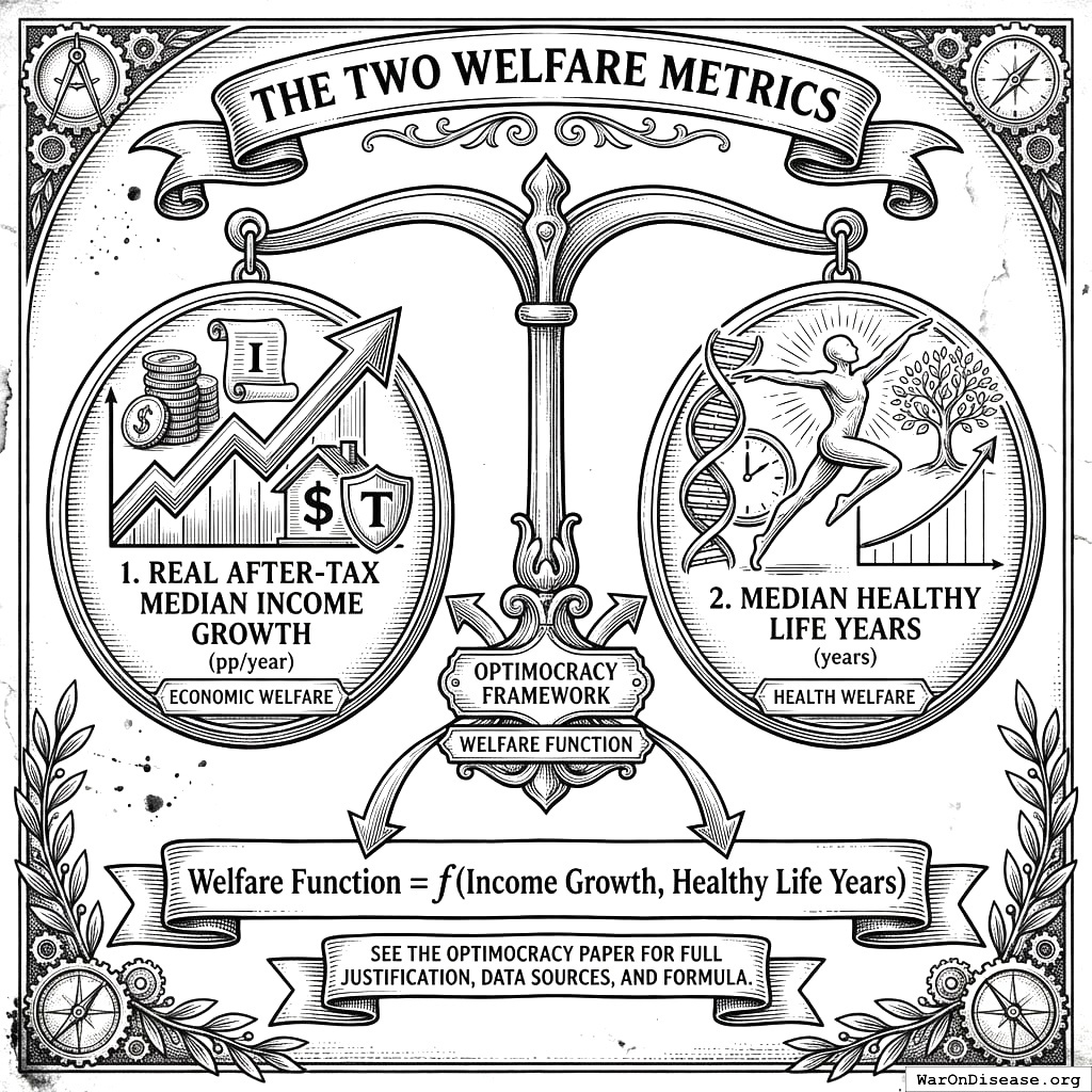
Real after-tax median income growth (pp/year) - economic welfare
Median healthy life years (years) - health welfare
See the Optimocracy paper for full justification of these metric choices, data sources, and the welfare function formula.
The two things that matter: having money and being alive to spend it. You’d think this would be obvious, but governments often forget the second bit.
1.1 Why Only Two Metrics?
Simplicity: These two metrics capture the primary welfare dimensions affected by most policies while remaining directly interpretable. No complex conversion factors (VSL, QALY→$) are needed.
Coverage gap: Freedom and autonomy concerns are handled as blocking factors rather than adding metric complexity. A policy that improves income and health but restricts freedom is flagged, not silently scored. Environmental impacts and distributional effects are tracked as supplementary indicators where data permits.
1.2 Income Metric Definition
Real after-tax median income growth is defined narrowly as: wages, salaries, and self-employment income, minus taxes paid. This metric captures what appears in household budgets.
What counts as income effects:
Wage increases from productivity gains (e.g., fewer sick days → measurably higher wages)
Tax changes that directly affect take-home pay
Employment effects that translate to wage income
What does NOT count as income effects:
Healthcare cost savings (these are health system efficiency gains, not personal income)
Reduced insurance premiums (unless they translate to higher take-home pay via employer pass-through)
Quality-of-life improvements that don’t appear in wages
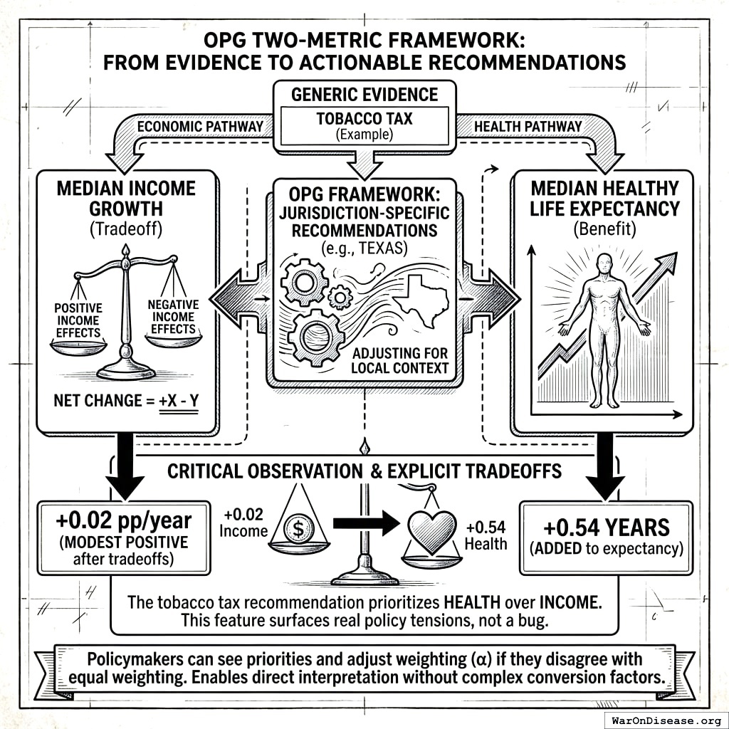
Implication for policy analysis: This creates genuine tradeoffs that the two-metric framework makes explicit. A tobacco tax, for example, may show:
Income effect: Negative for smokers (direct tax burden), partially offset by productivity gains for those who quit
Health effect: Positive (reduced smoking → longer healthy life)
The framework does not hide this tradeoff by claiming healthcare cost savings are “income gains.” If a policy improves health but costs money, both effects are reported honestly. This is a feature, not a bug: it prevents corner solutions (an infinite tobacco tax would maximize health but devastate income for smokers) and surfaces the welfare tradeoff for democratic deliberation.
1.3 Outcome Translation Methodology
While OPG uses only two terminal metrics (income growth and healthy life years), evidence often measures surrogate outcomes (smoking rates, traffic deaths, crime rates). This section specifies how surrogate outcomes are translated to the terminal metrics.
Where CV is the coefficient of variation at each translation step. A three-step translation with 30% uncertainty at each step yields ~52% uncertainty in the terminal metric.
Important clarification: The claim that “no complex conversion factors are needed” in the abstract refers to the terminal metrics themselves (income and health are directly interpretable, unlike utility or welfare indices). Translation from surrogate outcomes to terminal metrics does require conversion factors, which must be documented and include uncertainty bounds.
2 The Evidence Base: Centuries of Natural Policy Experiments
Every jurisdiction that enacted a policy created a natural experiment. The evidence to know what works already exists, scattered across thousands of jurisdictions and hundreds of years. OPG systematically harvests this evidence.
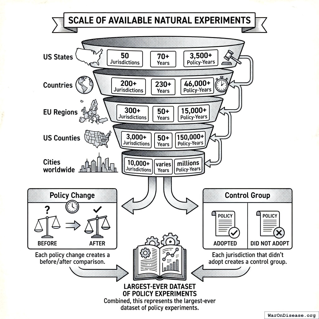
2.1 Scale of Available Natural Experiments
Level
Jurisdictions
Years
Policy-Years
US States
50
70+
3,500+
Countries
200+
230+
46,000+
EU Regions
300+
50+
15,000+
US Counties
3,000+
50+
150,000+
Cities worldwide
10,000+
varies
millions
Each policy change creates a before/after comparison. Each jurisdiction that didn’t adopt creates a control group. This represents a vast, largely untapped evidence base.
US states give you 3,500 policy-years of data. Cities worldwide give you millions. It’s like comparing a cookbook to the entire history of food.
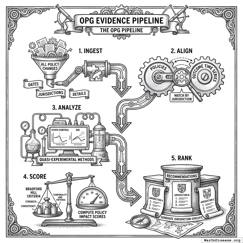
2.2 The OPG Pipeline
Data goes in, gets organized, analyzed, scored, then spits out recommendations. It’s a sausage factory, but for telling politicians what works instead of what kills you.
┌─────────────────────────────────────────────────────────────────┐
│                    OPG EVIDENCE PIPELINE                         │
├─────────────────────────────────────────────────────────────────┤
│                                                                  │
│  1. INGEST                                                       │
│     └── All policy changes with dates, jurisdictions, details   │
│                                                                  │
│  2. ALIGN                                                        │
│     └── Match policies to outcome time series by jurisdiction   │
│                                                                  │
│  3. ANALYZE                                                      │
│     └── Apply quasi-experimental methods (synth control, DiD)   │
│                                                                  │
│  4. SCORE                                                        │
│     └── Compute Policy Impact Scores using Bradford Hill        │
│                                                                  │
│  5. RANK                                                         │
│     └── Generate jurisdiction-specific recommendations          │
│                                                                  │
└─────────────────────────────────────────────────────────────────┘
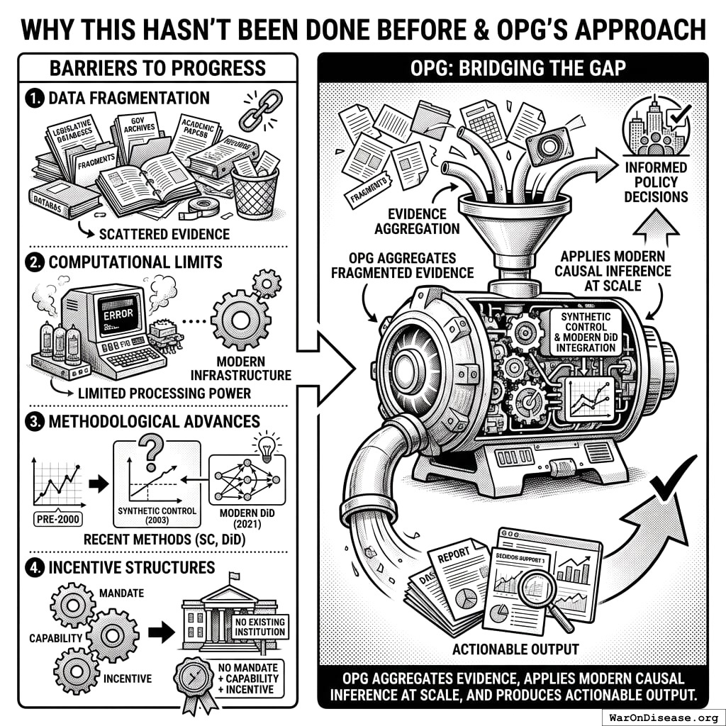
2.3 Why This Hasn’t Been Done Before
Data fragmentation: Policy records scattered across legislative databases, government archives, academic papers
Computational limits: Meta-analysis at this scale requires modern infrastructure
Methodological advances: Synthetic control (2003), modern DiD (2021) are recent
Incentive structures: No existing institution has mandate + capability + incentive
OPG aggregates fragmented evidence, applies modern causal inference at scale, and produces actionable output.
Four reasons this was impossible before: scattered data, slow computers, bad methods, nobody cared. Now: fast computers, good methods, some people care. Progress is three steps forward, four barriers removed.
3 System Overview
3.1 What Policymakers See
A jurisdiction-specific dashboard showing which policies to enact, replace, repeal, or maintain, ranked by expected welfare impact:
See Appendix A for a complete worked example showing jurisdiction-specific recommendations.
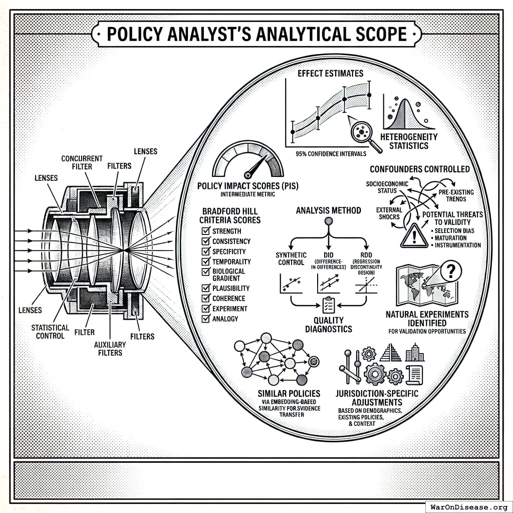
3.2 What Policy Analysts See
Eight different types of data combine to tell you if a policy actually works. Like ingredients in a recipe, except this one tells you which recipes poison people.
Effect estimates with standard errors, confidence intervals, and heterogeneity statistics
Policy Impact Scores (PIS) for each policy-outcome relationship (intermediate metric)
Bradford Hill criteria scores for causality assessment
Analysis method used (synthetic control, DiD, RDD) with quality diagnostics
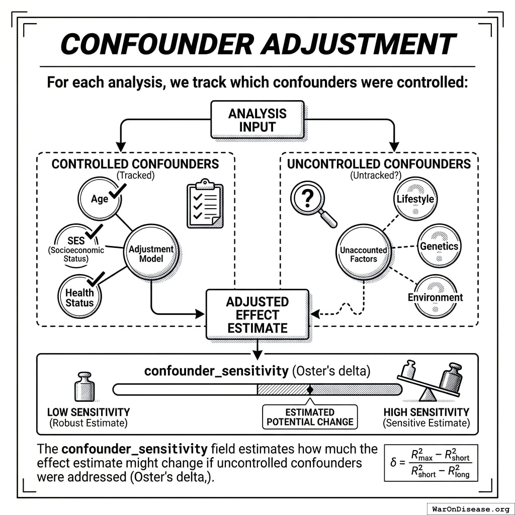
Confounders controlled and potential threats to validity
Natural experiments identified for validation opportunities
Jurisdiction-specific adjustments based on demographics, existing policies, and context
4 Introduction
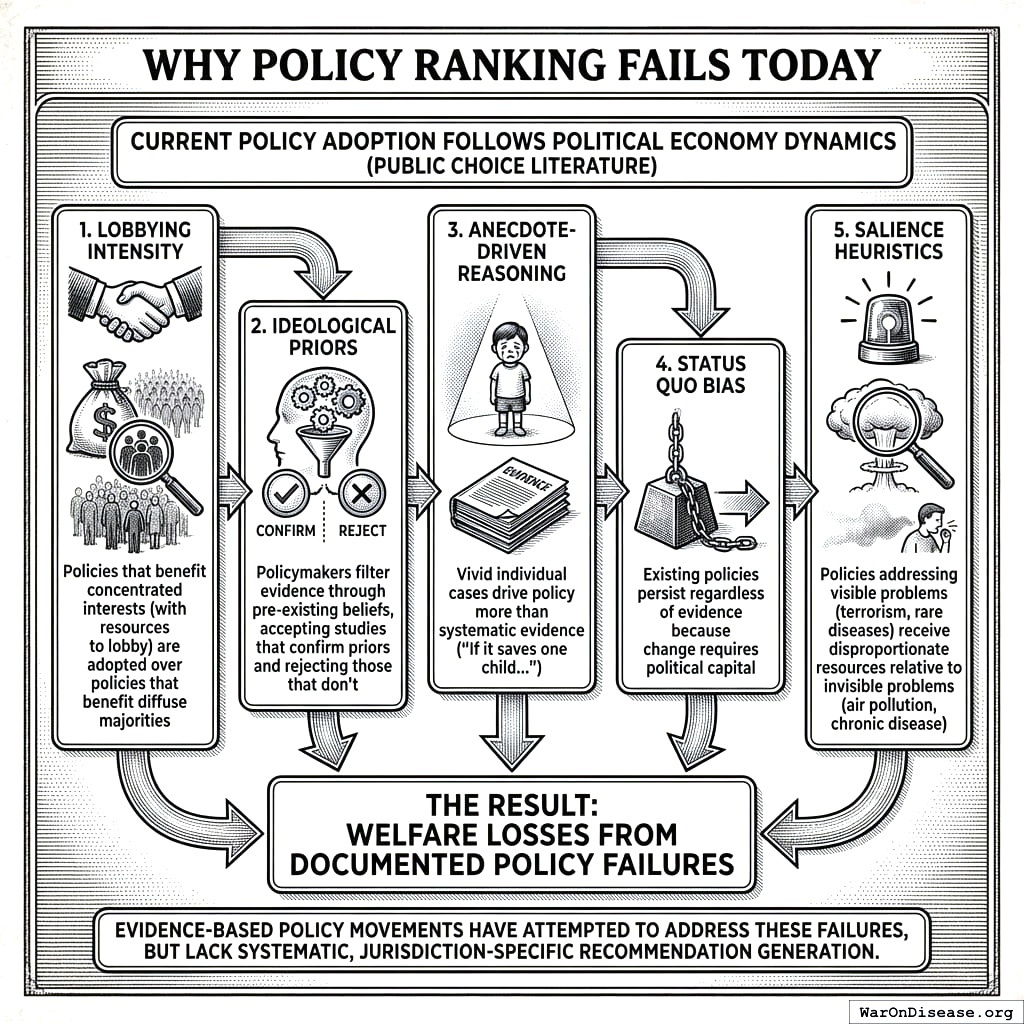
4.1 Why Policy Ranking Fails Today
Current policy adoption follows a process dominated by political economy dynamics well-documented in the public choice literature135,136:
Lobbying intensity: Policies that benefit concentrated interests (with resources to lobby) are adopted over policies that benefit diffuse majorities137,138
Ideological priors: Policymakers filter evidence through pre-existing beliefs, accepting studies that confirm priors and rejecting those that don’t
Anecdote-driven reasoning: Vivid individual cases drive policy more than systematic evidence (“If it saves one child…”)
Status quo bias: Existing policies persist regardless of evidence because change requires political capital
The result: welfare losses from documented policy failures. Evidence-based policy movements have attempted to address these failures139,140, but lack systematic, jurisdiction-specific recommendation generation.
Evidence says policy X works. But lobbying, fear of change, and shiny distractions filter it out. It’s like having the cure but drinking the poison because the bottle is prettier.
4.2 Scale of Available Evidence
The evidence base comprises millions of policy-years of natural experiments across all jurisdictional levels (see Section 2 for detailed counts). Even with imperfect causal inference, systematically analyzing this data should improve on the current system of lobbying-driven, ideology-filtered policy adoption. How much improvement is an empirical question requiring validation (see Section 20).
Current system: decide based on feelings, maybe 10 examples. New system: decide based on millions of examples. It’s the difference between astrology and astronomy, but for governance.
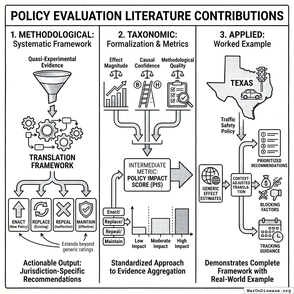
4.3 Contributions
Methodological: A systematic framework for translating quasi-experimental evidence into jurisdiction-specific policy recommendations, extending beyond generic evidence ratings to actionable output in four categories (enact/replace/repeal/maintain).
Evidence becomes a score. Score tells you: do this new thing, swap that old thing, stop doing that terrible thing, or keep doing that good thing. It’s like Marie Kondo, but for laws.
Taxonomic: We formalize the four recommendation types and introduce the Policy Impact Score (PIS) as an intermediate metric combining effect magnitude, causal confidence (Bradford Hill criteria), and methodological quality. This provides a standardized approach to evidence aggregation.
Applied: We demonstrate the complete framework with a worked example for Texas traffic safety policy, showing how generic effect estimates are translated into context-adjusted, prioritized recommendations with blocking factors and tracking guidance.
4.4 Validation Status
This specification describes a proposed framework. The methodology requires empirical validation before deployment. Specifically, retrospective studies should assess whether OPG-identified high-priority recommendations correlate with actual welfare improvements in jurisdictions that adopted them (see Section 20 for proposed validation design). Until such validation is completed, OPG outputs should inform but not replace expert judgment.
5 Related Work
5.1 Existing Policy Evaluation Frameworks
Regulatory Impact Analysis (RIA): Required by executive order for US federal regulations since 1981141. RIA estimates costs and benefits of proposed rules but: (1) applies only to new regulations, not the existing policy stock; (2) lacks systematic cross-jurisdiction evidence aggregation; (3) does not produce jurisdiction-specific recommendations for subnational governments.
What Works Clearinghouse (WWC): The Institute of Education Sciences operates WWC to review education interventions against methodological standards142. WWC demonstrates that systematic evidence synthesis is feasible, but: (1) covers only education; (2) provides generic intervention ratings, not jurisdiction-specific recommendations; (3) does not quantify expected welfare gains.
Cochrane and Campbell Collaborations: These systematic review organizations cover healthcare143 and social policy144 respectively. They represent the gold standard for evidence synthesis but: (1) produce narrative reviews rather than quantitative recommendations; (2) provide no jurisdiction-specific output; (3) operate on slow update cycles (years between reviews).
Congressional Budget Office (CBO): CBO provides nonpartisan fiscal scoring of proposed legislation. While valuable for budget discipline, CBO: (1) estimates budgetary effects rather than welfare; (2) evaluates what is proposed rather than what should be proposed; (3) is reactive rather than proactive.
Benefit-Cost Analysis Tradition: The broader benefit-cost literature145,146 provides theoretical foundations for policy evaluation but typically focuses on individual project or regulation assessment rather than systematic cross-jurisdiction recommendation generation.
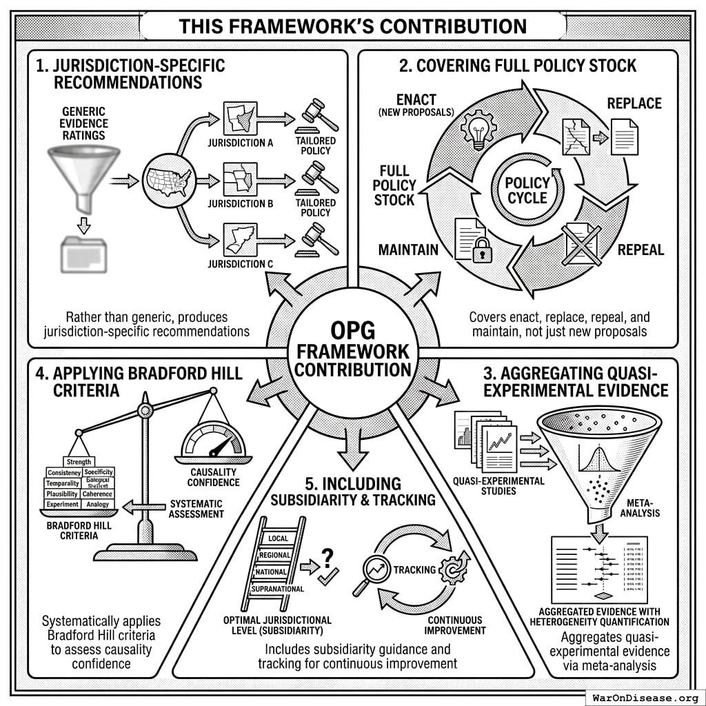
5.2 This Framework’s Contribution
How OPG is different from traditional evaluation: it’s personalized, comprehensive, and uses actual data instead of vibes.
OPG differs from existing approaches by:
Producing jurisdiction-specific recommendations rather than generic evidence ratings
Covering the full policy stock (enact/replace/repeal/maintain) not just new proposals
Aggregating quasi-experimental evidence via meta-analysis with heterogeneity quantification
Applying Bradford Hill criteria systematically to assess causality confidence
Including subsidiarity guidance (optimal jurisdictional level) and tracking for continuous improvement
6 Theoretical Framework
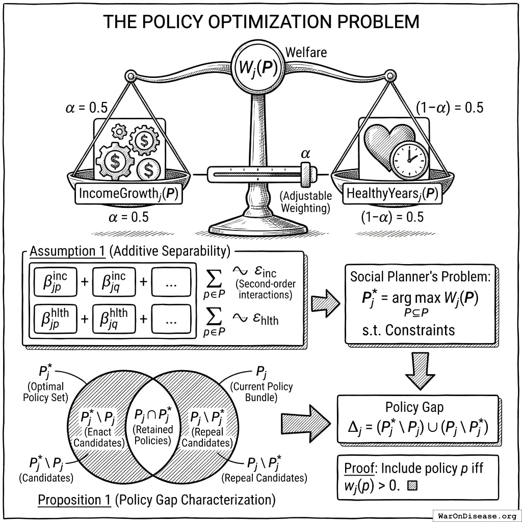
6.1 The Policy Optimization Problem
Let \(\mathcal{P}\) denote the set of available policies. For jurisdiction \(j\), let \(P_j \subseteq \mathcal{P}\) denote the current policy bundle. Welfare under policy bundle \(P\) is defined using the two core metrics:
\(\text{IncomeGrowth}_j(P)\) = Real after-tax median income growth (pp/year)
\(\text{HealthyYears}_j(P)\) = Median healthy life expectancy (years)
\(\alpha = 0.5\) (default equal weighting; can be adjusted for jurisdiction priorities)
The social planner’s problem: \[
P_j^* = \arg\max_{P \subseteq \mathcal{P}} W_j(P) \quad \text{subject to feasibility constraints}
\]
Assumption 1 (Additive Separability): For tractability, assume each metric is approximately additively separable across policies: \[
\text{IncomeGrowth}_j(P) \approx \sum_{p \in P} \beta^{\text{inc}}_{jp} + \varepsilon_{\text{inc}}
\]\[
\text{HealthyYears}_j(P) \approx \sum_{p \in P} \beta^{\text{hlth}}_{jp} + \varepsilon_{\text{hlth}}
\]
where \(\beta^{\text{inc}}_{jp}\) and \(\beta^{\text{hlth}}_{jp}\) are the marginal effects of policy \(p\) on each metric in jurisdiction \(j\), and interaction terms are assumed to be second-order.
Two circles: what you do now, what you should do. The bits that don’t overlap are where people are dying unnecessarily. Venn diagrams finally do something useful.
Justification and limitations: Additive separability is a standard simplifying assumption in policy analysis (see141 for regulatory impact analysis applications). This assumption is most valid when: (1) policies operate through distinct mechanisms, (2) jurisdictions have not reached saturation in any policy domain, and (3) policies do not create complementarities or substitution effects. When these conditions fail (for example, when a carbon tax interacts with renewable energy subsidies), the marginal effects may be mis-estimated.
Policy Interaction Detection:
OPG flags potential interaction effects using the following heuristics:
Effect heterogeneity test: If a policy’s effect varies significantly depending on whether another policy is present, flag the pair as potentially interacting.
Known interaction database: Documented policy complementarities and substitutes:
Policy A
Policy B
Interaction Type
Evidence
Seat belt law
Speed limit
Complementary
Both target crash fatalities
Nutrition labeling
School lunch programs
Complementary
Both improve dietary outcomes
Tobacco tax
Smoking ban
Complementary
Reinforce each other
Income tax cut
Sales tax increase
Substitutable
Offsetting fiscal effects
Sensitivity analysis recommendation: For high-priority recommendations, report: “How would this recommendation change if policies X and Y interact?” with bounds on combined effect.
Proposition 1 (Policy Gap Characterization): Under Assumption 1, the welfare-optimal policy set satisfies: \[
P_j^* = \{p \in \mathcal{P} : w_j(p) > 0\}
\]
and the policy gap for jurisdiction \(j\) is: \[
\Delta_j = (P_j^* \setminus P_j) \cup (P_j \setminus P_j^*)
\]
where \((P_j^* \setminus P_j)\) represents beneficial policies the jurisdiction lacks (enact candidates) and \((P_j \setminus P_j^*)\) represents harmful policies the jurisdiction has (repeal candidates). See Section 9 for the operational implementation.
Proof: Direct consequence of additive separability. Include policy \(p\) if and only if \(w_j(p) > 0\). ∎
6.2 Evidence Aggregation Properties
Proposition 2 (PIS as Precision-Weighted Evidence): Under random-effects meta-analysis with between-jurisdiction variance \(\tau^2\), the pooled effect estimate \(\hat{\beta}_{\text{pooled}}\) is (see Section 13 for implementation): \[
\hat{\beta}_{\text{pooled}} = \frac{\sum_j \frac{1}{\text{SE}_j^2 + \tau^2} \hat{\beta}_j}{\sum_j \frac{1}{\text{SE}_j^2 + \tau^2}}
\]
with variance: \[
\text{Var}(\hat{\beta}_{\text{pooled}}) = \frac{1}{\sum_j \frac{1}{\text{SE}_j^2 + \tau^2}}
\]
Proof: Standard random-effects meta-analysis derivation (DerSimonian-Laird). ∎
meaning the pooled estimate explains less than 25% of cross-jurisdiction variation. Context-specific estimates are required rather than direct application of the pooled effect. This constraint is operationalized in Section 13.4.
Proof: By definition, \(I^2 = \frac{\tau^2}{\tau^2 + \bar{\sigma}^2}\) where \(\bar{\sigma}^2\) is typical within-study variance. When \(I^2 > 0.75\), between-study variance dominates, and the pooled estimate provides limited information about any individual jurisdiction’s true effect. ∎
6.3 Information Value
Proposition 4 (Value of Additional Evidence): The expected value of information from an additional jurisdiction study is: \[
\text{VOI} = E[\max_{a \in \{adopt, reject\}} U(a | \text{new data})] - \max_{a} E[U(a | \text{current data})]
\]
which is maximized when prior uncertainty is high and decision stakes are large.
Corollary 1 (Trial Prioritization): Policies with (1) high prior variance in effect estimates, (2) large potential welfare impact, and (3) low trial cost should be prioritized for experimental validation. See Section 17 for implementation.
7 Core Methodology
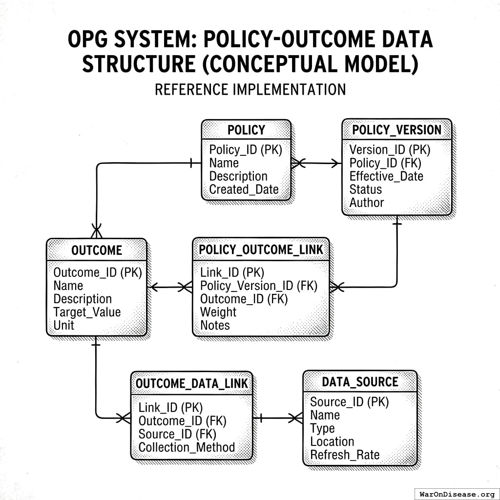
7.1 Policy-Outcome Data Structure
The OPG system uses a relational database schema. The following is a reference implementation showing the conceptual data model; production deployments may vary.
How the database connects policies to outcomes. It’s plumbing, but for knowledge instead of waste. Although some policies are also waste.
7.1.1 Core Tables
-- Hierarchical jurisdictions (country > state > county > city)jurisdictions (id, name, jurisdiction_type, -- 'country', 'state', 'county', 'city' parent_id, -- FK to parent jurisdiction (e.g., Texas -> USA) iso_code, population, gdp_per_capita, constitution_type, -- constraints on policy space data_quality_score, -- how complete is our policy inventory? latitude, longitude, ...)-- Policy types (canonical definitions)policy_types (id, name, policy_category_id, policy_type, is_continuous, typical_onset_delay_days, typical_duration_of_effect_years, canonical_text, ...)-- Current policy inventory by jurisdictionjurisdiction_policies ( jurisdiction_id, policy_type_id, has_policy BOOLEAN, policy_strength, -- e.g., tobacco tax amount, not just yes/no implementation_date, policy_details_json, data_source, last_verified)-- Two core welfare metrics (fixed schema)outcome_metrics (id, metric_type ENUM('income', 'health'), -- Only two types jurisdiction_id, measurement_date,value, -- pp/year for income; years for health confidence_interval_low, confidence_interval_high, data_source -- Census/BLS for income; WHO/BRFSS for health)-- Policy recommendations (generated output)policy_recommendations ( jurisdiction_id, policy_type_id, recommendation_type, -- 'enact', 'replace', 'repeal', 'maintain' current_status, -- what they have now (NULL if nothing) recommended_target, -- what evidence suggests-- Two-metric effects income_effect_pp, -- Expected effect on median income growth (pp/year) income_effect_ci_low, income_effect_ci_high, health_effect_years, -- Expected effect on healthy life years health_effect_ci_low, health_effect_ci_high, evidence_grade, priority_score, blocking_factors, -- 'constitutional', 'federal_preemption', 'political', 'autonomy', etc. similar_jurisdictions,-- Jurisdictional level guidance minimum_effective_level, recommended_level,-- Tracking for feedback loop tracking_frequency, tracking_baseline_method, last_generated)
7.1.2 Policy Types
Type
Description
Example
Measurement
law
Statutory law passed by legislature
Environmental regulation law
Binary (exists/not)
regulation
Administrative rule by agency
Agency emission standards
Continuous (stringency)
tax_policy
Tax rate, bracket, credit, deduction
Investment income tax rate
Continuous (rate)
budget_allocation
Spending decision
Education spending per pupil
Continuous ($/capita)
executive_order
Executive action
Enforcement priority directive
Binary
court_ruling
Judicial precedent
Constitutional interpretation
Binary
treaty
International agreement
Multilateral cooperation treaty
Binary
local_ordinance
Municipal rule
Land use restrictions
Categorical
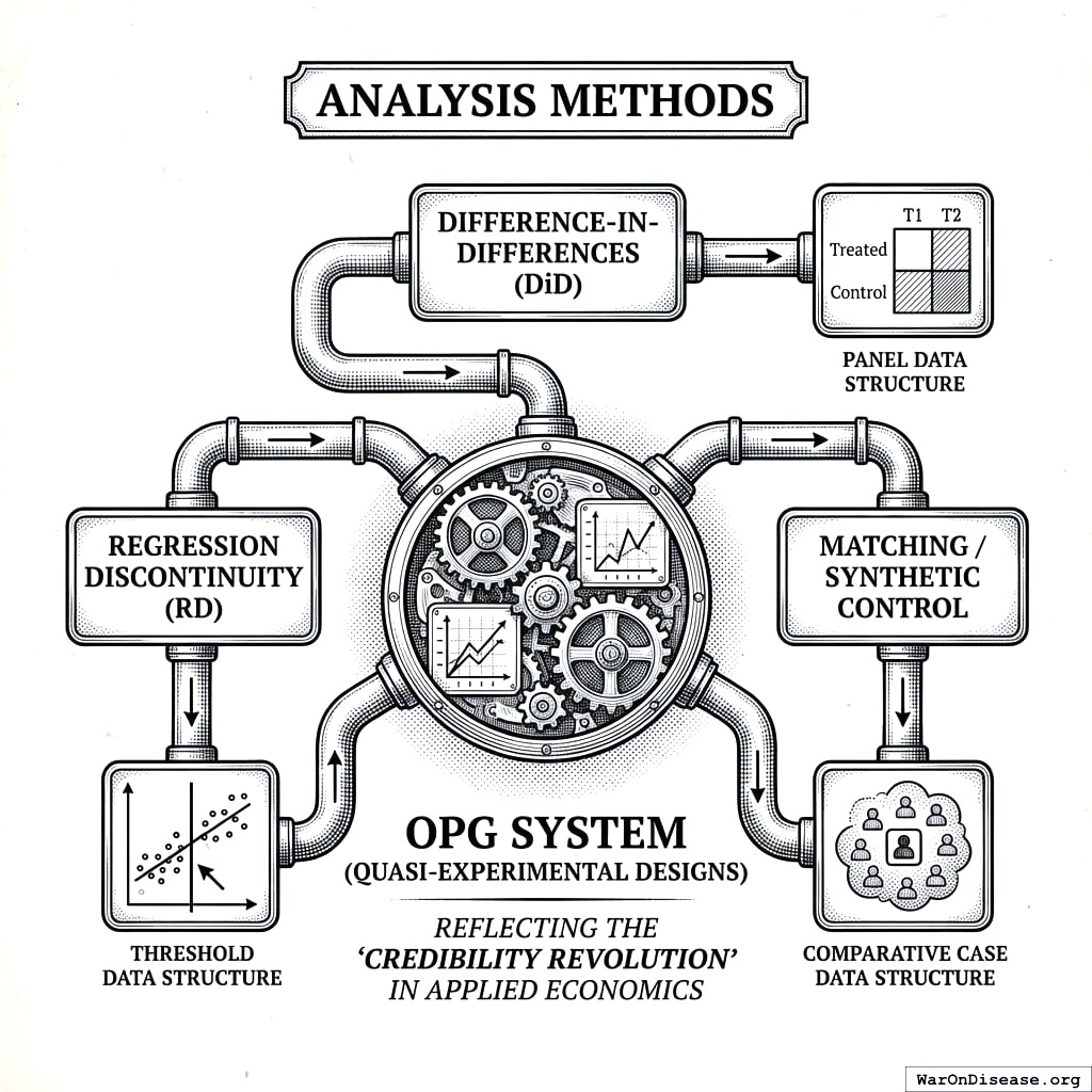
7.2 Analysis Methods
Different ways to figure out if policies work when you can’t run proper experiments because ethics committees get upset about randomly killing control groups.
The OPG system supports multiple quasi-experimental designs, reflecting the “credibility revolution” in applied economics147. Each method is appropriate for different data structures148:
7.2.1 Synthetic Control Method
Use case: Single treated jurisdiction, good donor pool of similar untreated jurisdictions.
Method: Construct a “synthetic” control as a weighted average of untreated jurisdictions that matches the treated jurisdiction’s pre-treatment outcome trajectory. Post-treatment divergence estimates the causal effect.
Quality metrics:
pre_treatment_rmse: How well does synthetic control match pre-treatment? (Lower is better)
placebo_p_value: Permutation test comparing treated effect to placebo effects (Lower is better)
Example: Effect of a state tobacco tax increase on smoking rates, using similar states without tax changes as donors149,150. For comprehensive reviews of the synthetic control method, see151.
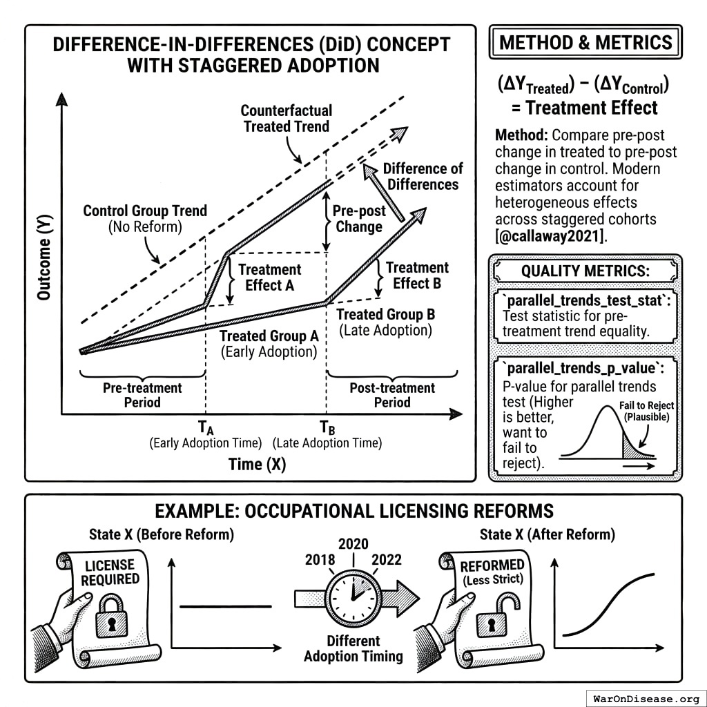
Two lines run parallel, then one gets the policy and diverges. The gap between them is how much the policy helped or hurt. It’s like twins, but one gets vegetables.
Method: Compare pre-post change in treated jurisdictions to pre-post change in control jurisdictions. Difference of differences estimates treatment effect. For settings with staggered adoption, modern estimators account for heterogeneous treatment effects across cohorts152.
Quality metrics:
parallel_trends_test_stat: Test statistic for pre-treatment trend equality
parallel_trends_p_value: P-value for parallel trends test (Higher is better, want to fail to reject)
Example: Effect of occupational licensing reforms across states with different adoption timing.
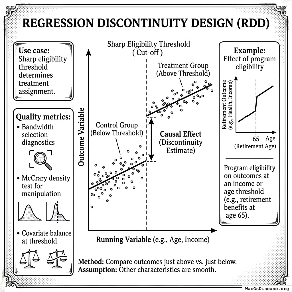
7.2.3 Regression Discontinuity Design (RDD)
Use case: Sharp eligibility threshold determines treatment assignment.
Dots on either side of a line, big jump at the cutoff. People just above the line do better. It’s like being born one day later and getting free healthcare.
Method: Compare outcomes just above vs. just below the threshold. If other characteristics are smooth across the threshold, the discontinuity in outcomes estimates the causal effect.
Quality metrics:
Bandwidth selection diagnostics
McCrary density test for manipulation
Covariate balance at threshold
Example: Effect of program eligibility on outcomes at an income or age threshold (e.g., retirement benefits at age 65).
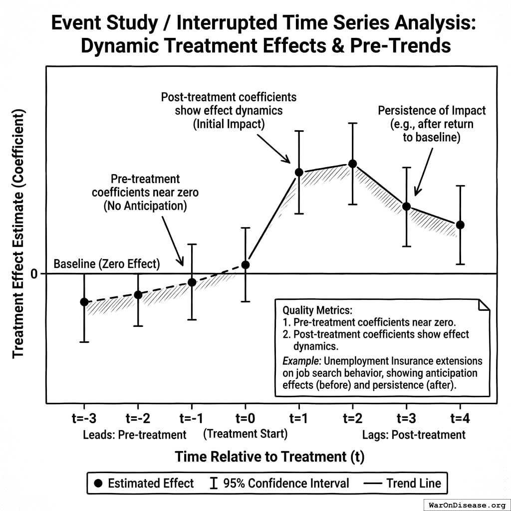
7.2.4 Event Study / Interrupted Time Series
Use case: Need to visualize pre-trends and dynamic treatment effects.
Nothing happens, nothing happens, nothing happens, policy hits, then things change. It’s like a heart rate monitor, but for legislation instead of life.
Method: Estimate treatment effects at each time period relative to treatment, including leads (pre-treatment) and lags (post-treatment).
Quality metrics:
Pre-treatment coefficients should be near zero (no anticipation)
Post-treatment coefficients show effect dynamics
Example: Effect of unemployment insurance extensions on job search behavior, showing both anticipation effects (before benefits expire) and persistence of impact (after return to baseline).
7.2.5 Confidence Weighting by Method
The following weights reflect proposed defaults based on the methodological rigor hierarchy in applied economics. These weights have not been empirically calibrated and should be treated as starting points for implementation.
Method
Base Confidence Weight
Rationale
Randomized experiment
1.00
Gold standard; rare for policies
Regression discontinuity
0.90
Local randomization at threshold
Synthetic control
0.85
Good pre-treatment fit implies validity
Difference-in-differences
0.80
Requires untestable parallel trends
Event study
0.75
Descriptive of dynamics; less rigorous
Interrupted time series
0.65
Single-unit; history threats
Simple before-after
0.40
No control group; confounding likely
Cross-sectional
0.25
Snapshot; severe confounding
7.3 Bradford Hill Criteria Scoring Functions
Bradford Hill’s criteria for causality153, originally developed for epidemiology, are operationalized here as explicit scoring functions. Each criterion maps to a saturation function that produces a score in \([0, 1]\).
Take nine different ways to check if something causes something else, squish them into numbers between 0 and 1. Science loves turning confidence into decimals.
7.3.1 Strength of Association
Larger effect estimates provide stronger evidence. We use an exponential saturation function:
Where \(|\hat{\beta}_{\text{std}}|\) is the absolute standardized effect size and \(\beta_{\text{sig}} = 0.3\) is the saturation parameter.
Parameter justification: The threshold \(\beta_{\text{sig}} = 0.3\) corresponds to Cohen’s convention for a “medium” effect size in social science154. This is a starting point; sensitivity analysis shows PIS changes by ±15% when \(\beta_{\text{sig}}\) varies from 0.2 to 0.4. A standardized effect of 0.3 yields \(S_{\text{strength}} \approx 0.63\); effects of 0.6+ yield scores \(>0.86\).
7.3.2 Consistency Across Jurisdictions
Replication across contexts provides stronger evidence. Scored by number of independent jurisdiction studies:
Where \(N_j\) is the number of jurisdictions with concordant effect direction and \(N_{\text{sig}} = 10\) is the saturation parameter.
Parameter justification: The threshold \(N_{\text{sig}} = 10\) reflects that replication across 10+ independent jurisdictions provides strong evidence against idiosyncratic local effects. This aligns with meta-analytic conventions where 10+ studies enable reliable heterogeneity estimation155. Sensitivity analysis shows PIS varies by ±12% when \(N_{\text{sig}}\) ranges from 7 to 15. Five concordant jurisdictions yield \(S_{\text{consistency}} \approx 0.39\); ten yield \(\approx 0.63\).
7.3.3 Temporality (Required)
Policy adoption must precede outcome change. This is binary (either satisfied or not):
Where \(\delta\) is the lag between policy implementation and outcome measurement. If temporality is violated, the overall CCS is zeroed regardless of other criteria.
Where \(r_{\text{dose}}\) is the correlation between policy intensity and outcome magnitude, and \(r_{\text{sig}} = 0.5\) is the saturation parameter.
Parameter justification: The threshold \(r_{\text{sig}} = 0.5\) reflects that a correlation of 0.5 between policy intensity and outcome represents moderate dose-response evidence. This is analogous to toxicological dose-response standards where monotonic relationships strengthen causal inference156. Sensitivity analysis shows PIS varies by ±8% when \(r_{\text{sig}}\) ranges from 0.3 to 0.7. A dose-response correlation of 0.5 yields \(S_{\text{gradient}} = 0.5\); correlation of 0.7 yields \(\approx 0.66\).
Binary policies: For binary (yes/no) policies, dose-response cannot be assessed. Rather than defaulting to a neutral score of 0.5, binary policies are marked as “N/A” for gradient and this criterion is excluded from the CCS calculation (weights are renormalized across remaining criteria). This prevents binary policies from being systematically penalized relative to continuous policies.
7.3.5 Experiment Quality
Quality of the quasi-experimental design, weighted by validity diagnostic violations:
Where \(w_{\text{method}}\) is the base method weight and \(v_{\text{violations}} \in [0, 1]\) is the proportion of validity checks failed (parallel trends, pre-treatment fit, placebo tests).
7.3.6 Plausibility (Mechanistic)
Economic or behavioral mechanism linking policy to outcome. Scored by expert-validated mechanism database:
Where \(m_i \in \{0, 1\}\) indicates whether mechanism component \(i\) is satisfied and \(w_i\) are component weights.
Mechanism component checklist:
Component
Weight
Assessment Criterion
Economic theory predicts direction
0.30
Peer-reviewed theory paper supports predicted sign
Behavioral response documented
0.25
Empirical evidence of behavioral change in response to similar policies
No implausible required assumptions
0.20
Mechanism doesn’t require assumptions contradicted by evidence
Timing consistent with mechanism
0.15
Effect onset matches expected mechanism timeline
Magnitude plausible
0.10
Effect size within range predicted by mechanism
Scoring procedure: Each component is scored binary (0 or 1) by literature review. The weighted sum yields \(S_{\text{plausibility}} \in [0, 1]\). When expert-validated mechanism assessments are unavailable, this score defaults to 0.5 with a note that mechanism plausibility is unassessed.
7.3.7 Coherence with Literature
Consistency with broader economic and social science evidence:
Where \(N_{\text{studies}}\) is the count of supporting studies in the literature and \(N_{\text{sig}} = 5\). Three supporting studies yield \(S_{\text{coherence}} \approx 0.45\); ten yield \(\approx 0.86\).
7.3.8 Specificity
Whether the policy affects specific outcomes rather than everything:
Where \(N_{\text{outcomes}}\) is the number of outcome categories with significant effects. A policy affecting 1-2 outcomes has \(S_{\text{specificity}} > 0.7\); a policy affecting 10+ outcomes has \(S_{\text{specificity}} < 0.3\). Lower specificity suggests confounding or measurement artifact.
7.4 Causal Confidence Score (CCS) Calculation
The aggregate CCS combines the eight non-temporality criteria with explicit weights, gated by temporality:
\(S_{\text{temporality}}\) acts as a binary gate: if temporality fails (policy doesn’t precede outcome), the entire CCS is zero regardless of other criteria scores.
Proposed default criterion weights:
These weights represent proposed defaults based on the relative importance of each criterion for causal inference in policy contexts. They can be adjusted based on domain expertise, sensitivity analysis, or empirical calibration. The weights are adapted from the epidemiological Bradford Hill framework and have not been empirically validated for policy applications.
Criterion
Weight
Role
Temporality
Gate
Binary prerequisite (must be 1.0 to proceed)
Experiment
0.225
Method quality is primary for causal inference
Consistency
0.19
Replication across jurisdictions crucial
Strength
0.15
Effect magnitude matters for welfare
Gradient
0.125
Dose-response is strong causal evidence
Coherence
0.10
Literature support adds confidence
Plausibility
0.09
Mechanism existence supports causation
Specificity
0.06
Targeted effects more credible
Analogy
0.06
Transfer learning from similar policies
Weights for the eight scored criteria sum to 1.0. Temporality is not weighted because it is a binary gate, not a continuous score.
8 Jurisdiction Policy Inventory
8.1 Tracking Current Policies by Jurisdiction
Before generating recommendations, OPG must know what policies each jurisdiction currently has. The jurisdiction_policies table tracks:
Field
Description
Example
has_policy
Whether jurisdiction has this policy type
TRUE/FALSE
policy_strength
For continuous policies, the current level
$1.41/pack (tobacco tax)
implementation_date
When current policy took effect
2009-01-01
policy_details_json
Structured details about implementation
{“primary_enforcement”: false}
data_source
Where this information came from
“Texas Tax Code §154.021”
last_verified
When this was last confirmed accurate
2024-06-15
8.2 Data Sources for Policy Status
Jurisdiction Level
Primary Sources
Update Frequency
Country
WTO, OECD, IMF policy databases
Annual
US State
NCSL, state legislative databases, LexisNexis
Continuous
EU Member
EUR-Lex, national legal databases
Continuous
US City/County
Municipal code databases, Municode
Varies
Other Subnational
National statistics offices, academic datasets
Varies
8.3 Handling Missing Data
Data completeness varies by jurisdiction and policy type:
Data Quality Score
Interpretation
Recommendation Confidence
> 0.9
Comprehensive inventory
Full confidence
0.7 - 0.9
Most major policies tracked
High confidence
0.5 - 0.7
Significant gaps
Medium confidence; flag gaps
< 0.5
Sparse data
Low confidence; prioritize data collection
Recommendations are only generated when policy status is known with reasonable confidence.
9 Policy Gap Analysis
9.1 Comparing Current to Optimal
For each jurisdiction \(j\), the policy gap for policy type \(p\) is:
\(|\text{Gap}_{jp}|\) = Absolute difference between evidence-supported and current policy level (normalized to \([0, 1]\))
\(\text{PIS}_p\) = Policy Impact Score (see Section 12), capturing effect magnitude and causal confidence
\(M_{jp}\) = Monetized annual welfare impact, adjusted for jurisdiction \(j\)’s population and context
Priority tiers:
Tier
Priority Score
Interpretation
Critical
\(\geq 0.80\)
Immediate action recommended
High
\([0.50, 0.80)\)
Strong candidate for adoption
Medium
\([0.25, 0.50)\)
Consider if political capital available
Low
\(< 0.25\)
Monitor for better evidence
High-priority recommendations have: 1. Large gap between current and optimal 2. Strong evidence (Grade A or B; high PIS) 3. Large expected welfare impact (high M)
9.4 Context Adjustment
Effect estimates are adjusted for jurisdiction characteristics:
This reflects increased uncertainty when extrapolating beyond the observed evidence distribution.
10 Recommendation Generation
10.1 Recommendation Types
Type
Question
When to Use
Example
Enact
“Add this?”
New policy the jurisdiction doesn’t have
“ENACT primary seat belt law”
Replace
“Change this?”
Modify existing policy level or approach
“REPLACE tobacco tax: $1.41 → $2.50”
Repeal
“Remove this?”
Remove policy with negative evidence
“REPEAL [harmful policy]”
Maintain
“Keep this?”
Current policy is evidence-supported
“MAINTAIN DUI threshold at 0.08 BAC”
For continuous policies (taxes, spending levels), Replace specifies the change from current to optimal level. Enact is reserved for truly new policies that don’t exist in the jurisdiction.
10.2 Blocking Factors
Recommendations flag constraints that may impede adoption:
Blocking Factor
Severity
Description
Example
Constitutional Constraint
Hard
Requires constitutional amendment
Takings Clause limits on land use regulations
Federal Preemption
Hard
Federal law prevents state/local action
Federal minimum wage floor
Treaty Obligation
Hard
International agreement constrains policy
WTO rules on tariffs
Autonomy Concern
Soft
Restricts individual freedom/choice
Mandatory helmet laws
Political Feasibility
Soft
Strong organized opposition
Industry lobbying
Implementation Cost
Soft
High fixed costs to implement
New regulatory agency needed
Design rationale: Why blocking factors are metadata only
OPG produces evidence-based rankings, not political forecasts. Blocking factors are flagged but do not affect algorithmic priority scores, for three reasons:
Political feasibility shifts over time. A policy “impossible” in 2020 may be mainstream by 2025. Filtering by current political feasibility would lock in the status quo and fail to surface the evidence-supported set.
Politicians know their context. An elected official in Texas understands local political dynamics better than any algorithm. OPG provides the evidence; filtering is left to policymaker judgment.
Autonomy tradeoffs require human judgment. A universal helmet law may save lives but restrict freedom. This is a value judgment, not an evidence question. OPG surfaces the health/income effects; the autonomy tradeoff is for democratic deliberation.
Hard vs. Soft blocking factors:
Hard blockers (constitutional, preemption, treaty): These represent legal impossibility at the current jurisdictional level. Recommendations with hard blockers are marked distinctly but still shown, as they may inform advocacy for constitutional change or higher-level policy.
Soft blockers (political, cost, autonomy): These represent practical difficulty, not impossibility. Many transformative policies faced “impossible” political opposition before adoption.
Important: The full evidence-supported recommendation set is always shown. Users can filter by blocking factor severity if desired, but the default view shows all recommendations ranked by expected welfare impact.
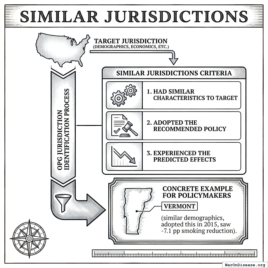
10.3 Similar Jurisdictions
For each recommendation, OPG identifies jurisdictions that: 1. Had similar characteristics to the target jurisdiction 2. Adopted the recommended policy 3. Experienced the predicted effects
This provides concrete examples for policymakers: “Vermont (similar demographics, adopted this in 2015, saw -7.1 pp smoking reduction).”
How to find good examples to copy: find places like you, who did the thing, and didn’t collapse. It’s like plagiarism, but encouraged.
10.3.1 Computing Jurisdiction Similarity
Similarity between jurisdictions \(j_1\) and \(j_2\) is computed as a weighted sum across three dimensions:
Where \(z\) values are z-scores and the denominator normalizes to [0,1] (4 SD maximum difference).
Institutional Similarity (\(\text{sim}_I\)):
Feature
Comparison
Federal vs. unitary
Binary match (1.0 if same, 0.5 if different)
Legal tradition
Common law, civil law, mixed (1.0/0.5/0.0)
Enforcement capacity
World Bank governance indicator proximity
Corruption level
Transparency International CPI proximity
Usage: Jurisdictions with \(\text{sim}(j_1, j_2) > 0.7\) are considered “similar” for evidence transfer purposes. Effect estimates from similar jurisdictions receive higher weight in context adjustment.
10.4 Recommended Tracking (for OPG Feedback)
Each recommendation includes minimal tracking guidance to enable continuous OPG improvement:
Field
Description
Example
Primary metric
The outcome variable to track
Traffic deaths per 100K
Data source
Where to get it
State vital statistics
Measurement frequency
How often
Annual
Comparison baseline
What to compare against
Pre-implementation 3-year average
This creates a learning loop: OPG recommends → jurisdiction implements → reports outcomes → OPG improves future recommendations.
OPG suggests thing, place does thing, place reports how it went, OPG learns. It’s a feedback loop, except it actually uses the feedback instead of filing it.
11 Optimal Jurisdictional Level for Policy Implementation
11.1 The Subsidiarity Principle for Evidence Generation
OPG recommends policies be implemented at the lowest jurisdictional level where the policy can be effective, for two reasons:
Maximize experimental data: 50 states experimenting > 1 federal policy. 3,000+ counties > 50 states. More jurisdictions = more natural experiments = faster evidence accumulation.
Federal level: little data, big risk. County level: lots of data, small risk. It’s safer to experiment in Shropshire than with the entire country.
Minimize harm from policy failures: A failed city ordinance affects thousands; a failed federal policy affects hundreds of millions. Lower-level experimentation bounds downside risk.
11.2 When Higher Levels Are Necessary
Some policies require higher jurisdictional levels:
Reason
Example
Recommendation
Externalities
Pollution crosses borders
State or federal
Race-to-bottom risk
Labor standards, tax competition
Federal floor, state variation above
Network effects
Infrastructure standards
Federal coordination
Economies of scale
Defense, diplomacy
National
11.3 Jurisdictional Level in Recommendations
For each policy recommendation, OPG specifies:
Field
Example
Minimum effective level
“City or higher”
Recommended level
“City (maximize data collection)”
Current adoption
“12 states, 47 cities have this”
Level constraints
“Federal preemption prevents city-level”
12 Policy Impact Score (Intermediate Metric)
12.1 Overview
The Policy Impact Score (PIS) is the intermediate metric used to generate recommendations. It quantifies the strength of evidence that a policy affects an outcome, combining effect magnitude, causal confidence, and analysis quality into a single score.
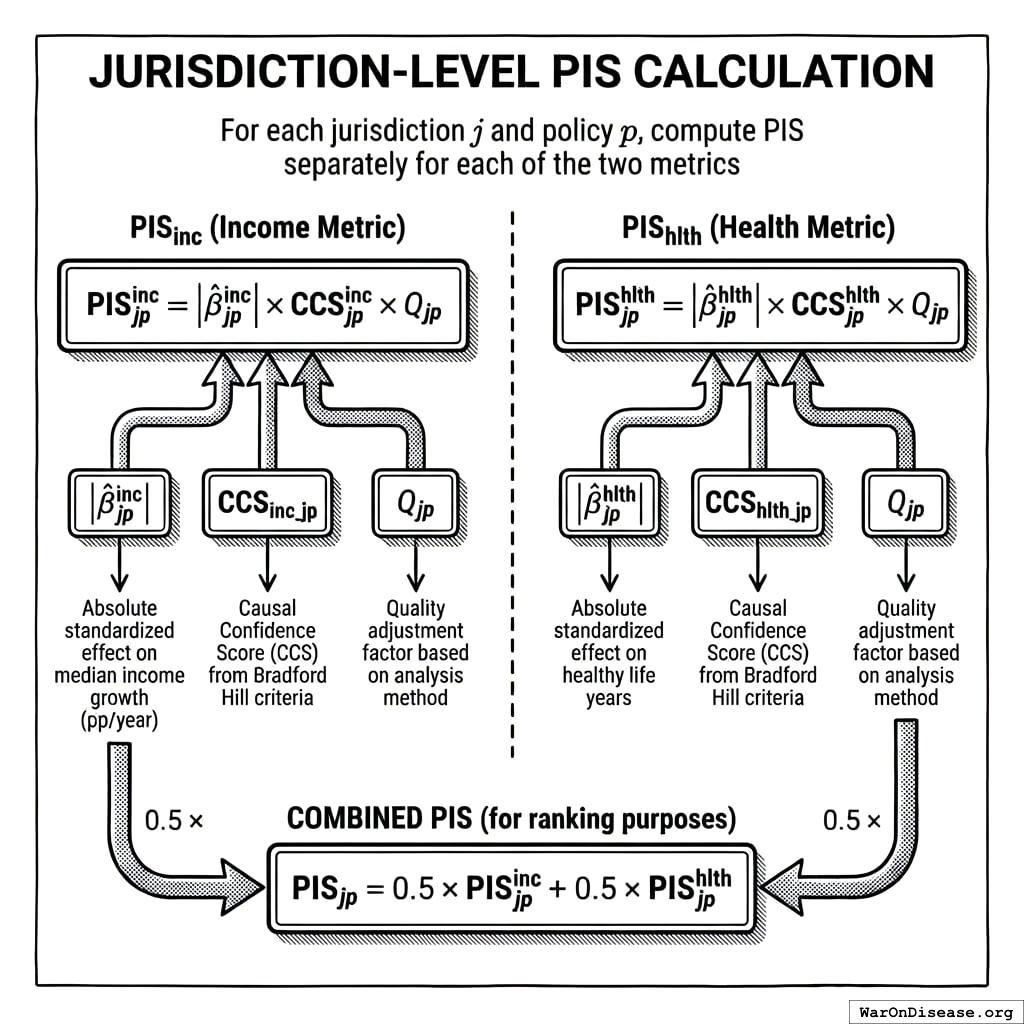
12.2 Jurisdiction-Level PIS Calculation
How to calculate if a policy works: add up how big the effect is, how sure we are, and how good the data is, for both money and health. Then argue about the number.
For each jurisdiction \(j\) and policy \(p\), compute PIS separately for each of the two metrics:
Where \(\sigma_{\text{income}}\) is the cross-jurisdictional SD of median income growth (typically ~1.5 pp/year) and \(\sigma_{\text{health}}\) is the cross-jurisdictional SD of healthy life expectancy (typically ~3-5 years).
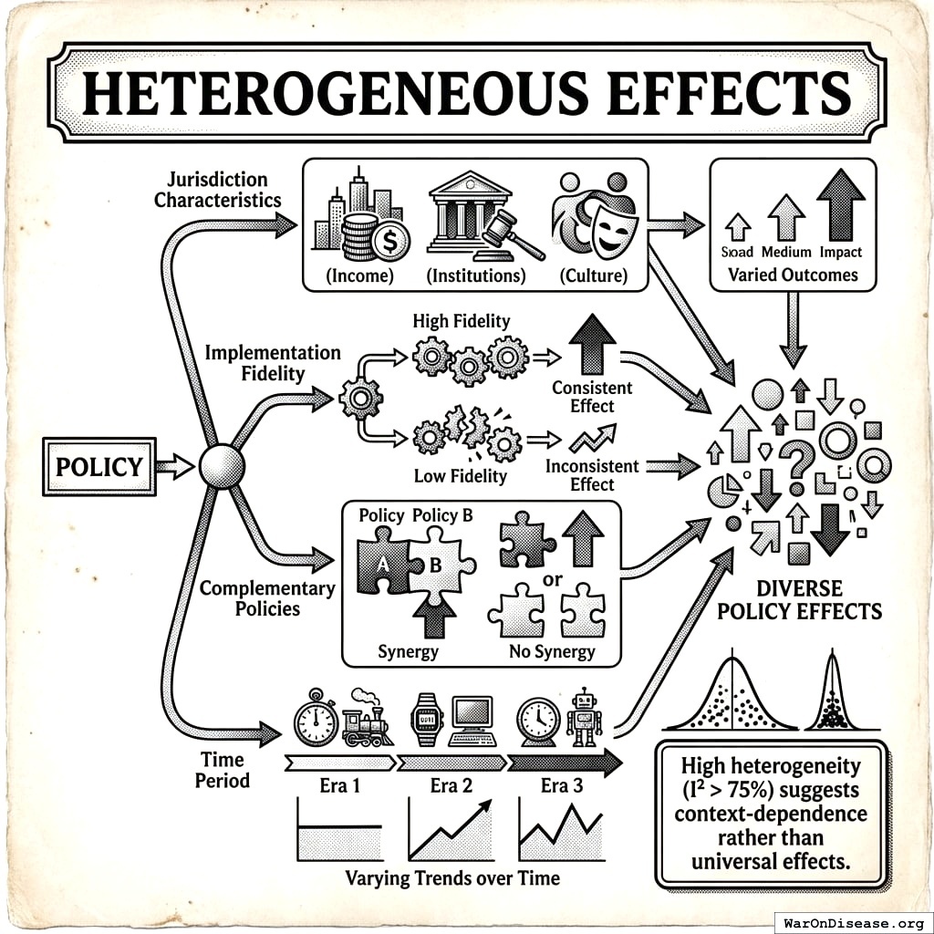
I²: Percentage of variance due to heterogeneity (vs. sampling error)
\(I^2 < 25\%\): Low heterogeneity
\(25\% \leq I^2 < 75\%\): Moderate heterogeneity
\(I^2 \geq 75\%\): High heterogeneity (effects vary substantially across jurisdictions)
τ²: Estimated between-study variance
Q statistic: Cochran’s test for heterogeneity
High heterogeneity suggests moderators (policy effects vary by context) rather than a single true effect.
13.4 Evidence Grading
Evidence grades are assigned using explicit thresholds on PIS, heterogeneity (\(I^2\)), and jurisdiction count (\(N_j\)):
\[
\text{Grade} = \begin{cases}
A & \text{if } \text{PIS} \geq 0.80 \text{ AND } I^2 < 0.50 \text{ AND } N_j \geq 5 \\
B & \text{if } \text{PIS} \geq 0.60 \text{ AND } I^2 < 0.50 \text{ AND } N_j \geq 3 \\
C & \text{if } \text{PIS} \geq 0.40 \text{ AND } I^2 < 0.75 \text{ AND } N_j \geq 2 \\
D & \text{if } \text{PIS} \geq 0.20 \\
F & \text{otherwise}
\end{cases}
\]
Grade interpretation:
Grade
PIS Threshold
Heterogeneity
Jurisdictions
Interpretation
A
\(\geq 0.80\)
\(I^2 < 50\%\)
\(\geq 5\)
Strong evidence; ready for implementation
B
\(\geq 0.60\)
\(I^2 < 50\%\)
\(\geq 3\)
Good evidence; consider piloting
C
\(\geq 0.40\)
\(I^2 < 75\%\)
\(\geq 2\)
Suggestive evidence; needs validation
D
\(\geq 0.20\)
Any
Any
Weak evidence; exploratory only
F
\(< 0.20\)
Any
Any
Insufficient evidence
Threshold calibration methodology:
These thresholds are proposed defaults requiring retrospective calibration. The calibration procedure:
Historical validation: Apply OPG grading to policies adopted 10+ years ago with known outcomes
Target validation rates: Grade A recommendations should validate at 70%+ rate; Grade B at 50%+
Threshold adjustment: If observed validation rates differ from targets, adjust PIS and \(I^2\) thresholds
Heterogeneity threshold rationale:
The \(I^2 < 50\%\) threshold for Grades A and B follows Cochrane Collaboration guidance that heterogeneity above 50% indicates “substantial” variability across studies143. Grade C allows heterogeneity up to 75% (the “high” threshold) with explicit acknowledgment that effects are context-dependent. Above 75%, pooled estimates provide limited guidance for any specific jurisdiction.
Evidence grading decision rule (text summary): start with PIS threshold, then apply heterogeneity threshold (\(I^2\)), then jurisdiction count (\(N_j\)). The canonical Grade A/B threshold in this spec is \(I^2 < 50\%\).
Additional grade modifiers:
Conflicting evidence: Downgrade by 1 letter if direction of effect differs across high-quality studies
High-quality RCT: Automatic Grade A if RCT with low risk of bias, regardless of other criteria
Single jurisdiction: Maximum Grade C unless effect is extraordinarily large (\(|\hat{\beta}| > 1.0\) SD)
13.5 Context-Specific Confidence
Effects may vary by jurisdiction characteristics. We report confidence separately for:
Context
Description
Example Modifier
High-income countries
OECD members, GDP/capita > $30K
Tax policy effects
Low-income countries
GDP/capita < $5K
Different institutional capacity
Federal systems
Policy set at national level
vs. subnational variation
Subnational
States, provinces, cities
Local policy autonomy
14 Quality Requirements & Validation
14.1 Minimum Thresholds for Inclusion
Criterion
Minimum
Rationale
Pre-treatment periods
4
Need to assess pre-trends
Post-treatment periods
2
Need to observe effect
Outcome observations
20
Statistical power
Control jurisdictions (for DiD)
5
Donor pool size
Pre-treatment RMSE (synthetic control)
< 2 SD
Acceptable pre-treatment fit
14.2 Parallel Trends Testing (DiD)
For difference-in-differences analyses, we test whether treated and control jurisdictions had parallel outcome trends before treatment:
Estimate event study with pre-treatment leads
Test joint significance of pre-treatment coefficients
If p < 0.10, flag as potential parallel trends violation
Report sensitivity: how different would trends need to be to explain away the effect?
Parallel trends test workflow: estimate event-study leads, run a joint significance test on pre-treatment leads, flag when \(p < 0.10\), then report sensitivity to plausible alternative trends.
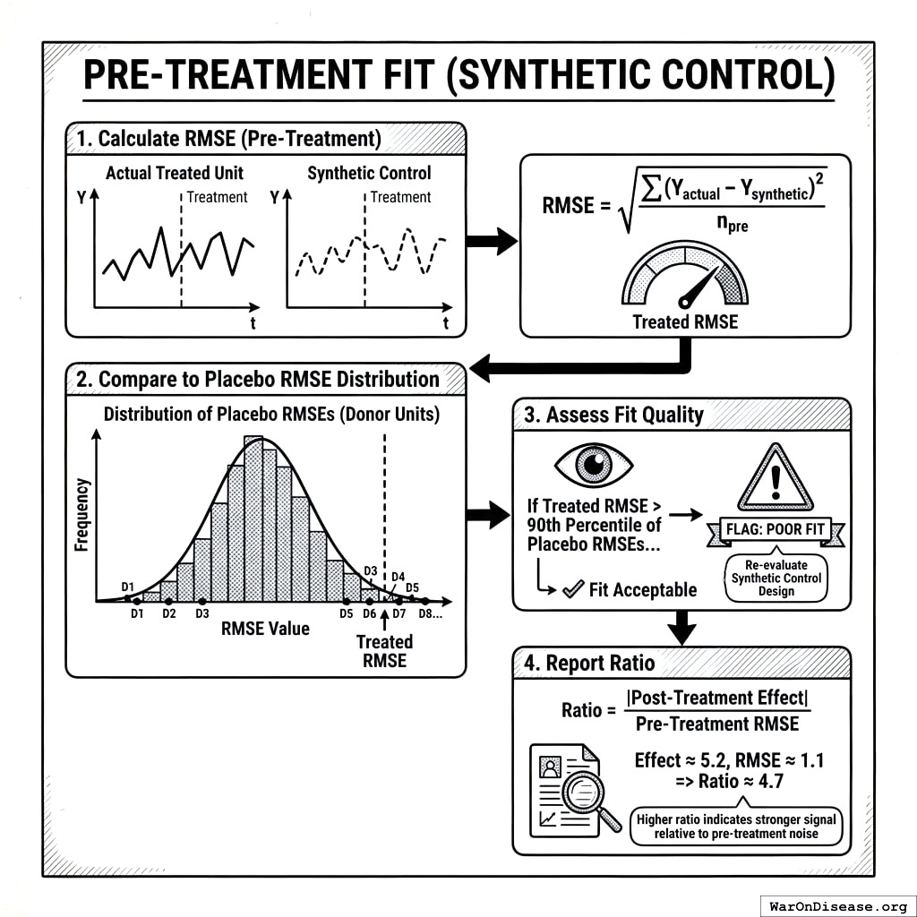
14.3 Pre-Treatment Fit (Synthetic Control)
How to check if your fake control group is good enough: measure error, try fake treatments, reject if it’s rubbish. Quality control for imaginary things.
For synthetic control analyses:
Calculate RMSE of synthetic vs. actual treated unit pre-treatment
Compare to distribution of placebo RMSEs (treating each donor as “treated”)
If treated RMSE is in top 10% of placebo RMSEs, flag as poor fit
Report ratio of post-treatment effect to pre-treatment RMSE
14.4 Placebo and Robustness Tests
Test
Purpose
Implementation
In-time placebo
Does “treatment” show effect before it happened?
Assign fake treatment date before actual
In-space placebo
Do untreated units show similar effects?
Apply analysis to control jurisdictions
Leave-one-out
Is result driven by single jurisdiction?
Re-estimate dropping each jurisdiction
Bandwidth sensitivity
(For RDD) Is result robust to bandwidth choice?
Estimate with multiple bandwidths
Covariate adjustment
Does controlling for confounders change result?
Add covariates, compare estimates
15 Interpreting Recommendations
15.1 Priority Tiers
Tier
Criteria
Action
Quick Wins
High impact, low blocking factors, Grade A evidence
Immediate adoption recommended
Major Reforms
High impact, significant blocking factors
Requires political capital; strategic timing
Long-Term
Moderate impact, constitutional or treaty constraints
Requires structural change
Monitor
Moderate impact, Grade C/D evidence
Watch for better evidence
15.2 Political Feasibility Notes
While OPG does not filter by political feasibility, it provides context:
Organized opposition: Industries or groups likely to lobby against
Public opinion: Polling data on similar policies where available
Adjacent jurisdictions: Whether neighbors have adopted (diffusion effects)
Historical attempts: Previous failed attempts and why
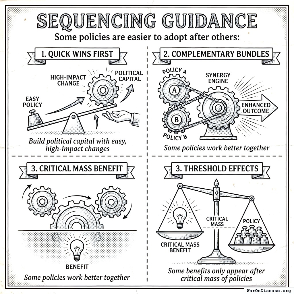
15.3 Sequencing Guidance
Start with easy wins, build momentum, bundle things together, hit critical mass. It’s like a diet plan, but for governance and with better success rates.
Some policies are easier to adopt after others:
Quick wins first: Build political capital with easy, high-impact changes
Complementary bundles: Some policies work better together
Threshold effects: Some benefits only appear after critical mass of policies
16 Effect Size Benchmarks
Effect sizes are calibrated to cross-jurisdictional variation to aid interpretation:
Size
Income (pp/year)
Health (years)
Example
Small
< 0.05
< 0.1
Minor regulatory changes
Medium
0.05 - 0.15
0.1 - 0.3
Typical tax policy effects
Large
0.15 - 0.30
0.3 - 0.5
Major reform programs
Very Large
> 0.30
> 0.5
Transformative policies (rare)
Calibration basis: US states vary by ~1.5 pp/year in median income growth and ~3-5 years in healthy life expectancy. A “medium” effect represents ~10% of cross-state variation.
Confidence interval interpretation:
Narrow (< 25% of effect): Precise estimate; high confidence
Moderate (25-50% of effect): Reasonable precision
Wide (> 50% of effect): Imprecise; low confidence
For the complete two-metric framework definition, see Section 1.
17 Trial Prioritization
17.1 Value of Information Calculation
The expected value of running a randomized trial on policy \(p\) is:
High heterogeneity (I² > 75%) suggests context-dependence rather than universal effects.
Same policy, different places, different results. Turns out context matters. Who knew, apart from everyone who’s ever tried anything anywhere.
19.4 Jurisdiction-Specific Caveats
Caveat
Description
Mitigation
Data completeness
Policy inventory may be incomplete
Flag data quality; recommend verification
Context transfer
Effect in State A may not transfer to State B
Adjust for observable differences; widen CIs
Implementation variation
Same policy, different enforcement
Track implementation quality where possible
Interaction effects
Effect depends on other policies in place
Model policy bundles, not just single policies
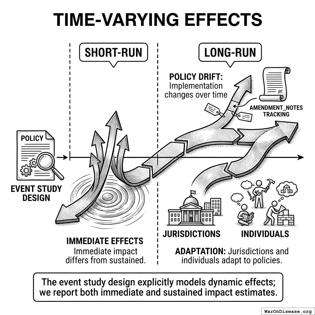
19.5 Time-Varying Effects
Short-run vs. long-run: Immediate effects may differ from sustained effects
Policy drift: Implementation changes over time (amendment_notes tracking)
Adaptation: Jurisdictions and individuals adapt to policies
The event study design explicitly models dynamic effects; we report both immediate and sustained impact estimates.
Immediate effect, people adapt, effect drifts, long-run effect settles. Policies age like milk, not wine.
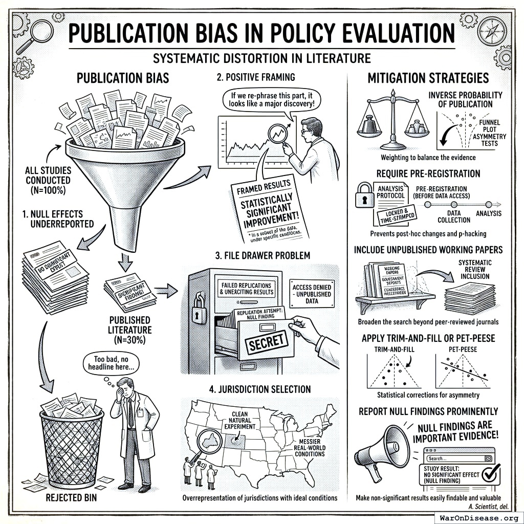
19.6 Publication Bias
Studies that find nothing don’t get published, so we think everything works. Funnel plots fish the failures out of the file drawer. Science learns to count its zeros.
The policy evaluation literature suffers from systematic publication bias:
Null effects underreported: Studies finding “no significant effect” are less likely to be published
Positive framing: Researchers may frame results to emphasize statistically significant findings
File drawer problem: Failed replications rarely published
Jurisdiction selection: Jurisdictions with cleaner natural experiments are overrepresented
Mitigation strategies:
Weight by inverse probability of publication (using funnel plot asymmetry tests)
Require pre-registration of analysis protocols before data access
Include unpublished working papers and government reports
Apply trim-and-fill or PET-PEESE corrections for funnel plot asymmetry
Report null findings prominently in the database
19.7 Epistemic Limitations
OPG provides evidence-weighted recommendations, not causal proof:
What OPG Can Do
What OPG Cannot Do
Rank policies by strength of quasi-experimental evidence
Prove any policy causes an outcome
Generate jurisdiction-specific recommendations
Guarantee effects transfer to new contexts
Identify promising candidates for randomized pilots
Replace randomized policy experiments
Quantify uncertainty and heterogeneity
Eliminate unmeasured confounding
Flag potential harms with moderate confidence
Guarantee a policy is safe
Transfer evidence across similar jurisdictions
Account for all local factors
Important: The quasi-experimental methods used provide evidence consistent with causation under assumptions that are often untestable. Synthetic control assumes the donor pool adequately represents the counterfactual; difference-in-differences assumes parallel trends would have continued; regression discontinuity assumes no manipulation around the threshold. These assumptions cannot be verified from data alone.
20 Validation Framework
20.1 The Critical Question
The ultimate test of OPG validity: Do jurisdictions that adopt high-priority OPG recommendations see better outcomes than those that don’t?
20.2 Addressing Adoption Bias
A naive retrospective comparison suffers from adoption bias: jurisdictions that voluntarily adopt policies may differ systematically from those that don’t. States adopting tobacco tax increases may already have anti-smoking momentum, overstating the causal effect of the tax itself.
Instrumental variable approach:
To address adoption bias, validation should exploit exogenous shocks to adoption:
Exogenous Shock
Example
Rationale
Court rulings
State court strikes down previous policy
Adoption forced by legal ruling, not political choice
Federal mandates
Clean Air Act state implementation
Compliance driven by federal law, not state preference
Close electoral outcomes
Ballot measure passes 51-49%
Near-randomization around threshold
Leadership turnover
New governor from different party
Adoption reflects leadership change, not underlying trends
These quasi-random adoption events provide cleaner tests of OPG predictions than voluntary adoption comparisons.
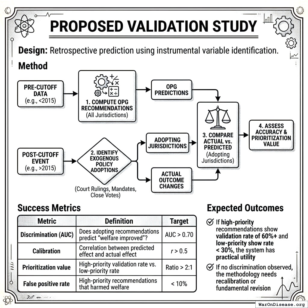
20.3 Proposed Validation Study
Design: Retrospective prediction using instrumental variable identification.
Check if the system would have been right in the past: compute old data, identify policies, compare predictions to reality, grade yourself. It’s like marking your own homework, but honest.
Method:
Compute OPG recommendations for all jurisdictions using only data available before a cutoff date (e.g., 2015)
Identify exogenously-induced policy adoptions (court rulings, mandates, close votes) after the cutoff
Compare actual outcome changes in adopting jurisdictions to OPG predictions
Assess prediction accuracy and prioritization value
Success Metrics (strengthened from initial draft):
Metric
Definition
Target
Discrimination (AUC)
Does adopting recommendations predict “welfare improved”?
AUC > 0.70
Calibration
Correlation between predicted effect and actual effect
r > 0.5
Prioritization value
High-priority validation rate vs. low-priority rate
Ratio > 2:1
False positive rate
High-priority recommendations that harmed welfare
< 10%
Expected Outcomes:
If high-priority recommendations show validation rate of 60%+ and low-priority show rate < 30%, the system has practical utility
If no discrimination observed, the methodology needs recalibration or fundamental revision
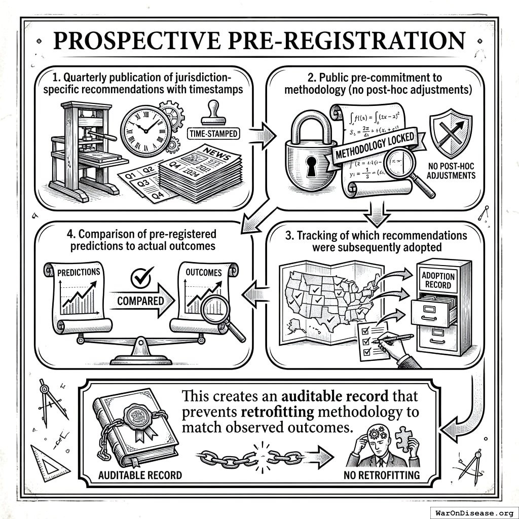
20.4 Prospective Pre-Registration
To prevent hindsight bias, OPG should publish recommendations before adoption decisions are made:
Quarterly publication of jurisdiction-specific recommendations with timestamps
Public pre-commitment to methodology (no post-hoc adjustments)
Tracking of which recommendations were subsequently adopted
Comparison of pre-registered predictions to actual outcomes
This creates an auditable record that prevents retrofitting methodology to match observed outcomes.
Promise what you’ll measure before you measure it, then stick to the promise. Prevents ‘we meant to test that all along’ syndrome.
20.5 Known Limitations Requiring Validation
Context adjustment accuracy: Do jurisdiction-specific adjustments improve prediction?
Blocking factor impact: Are recommendations with blocking factors less likely to be adopted?
Evidence grade thresholds: Are the A-F grade cutoffs appropriately calibrated?
Heterogeneity interpretation: Does high I² actually indicate context-dependence vs. measurement noise?
Translation pipeline accuracy: Do surrogate→terminal metric conversions introduce systematic bias?
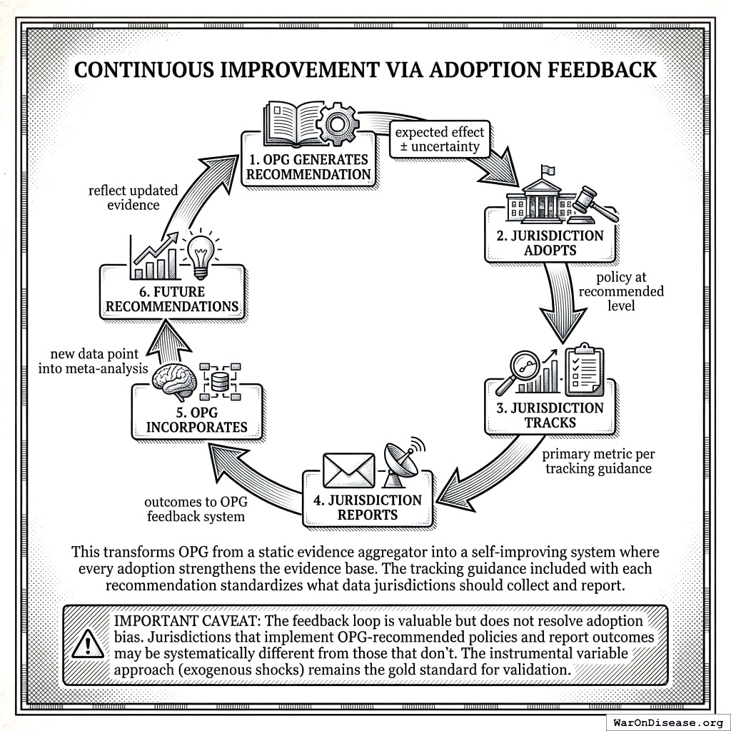
20.6 Continuous Improvement via Adoption Feedback
OPG improves through a learning loop:
OPG generates recommendation with expected effect ± uncertainty
Jurisdiction adopts policy at recommended level
Jurisdiction tracks primary metric per tracking guidance
Jurisdiction reports outcomes to OPG feedback system
OPG incorporates new data point into meta-analysis
Future recommendations reflect updated evidence
This transforms OPG from a static evidence aggregator into a self-improving system where every adoption strengthens the evidence base. The tracking guidance included with each recommendation standardizes what data jurisdictions should collect and report.
Recommend policy, place tries it, place reports results, analysis updates, better recommendations. It’s machine learning, but for government instead of cat pictures.
Important caveat: The feedback loop is valuable but does not resolve adoption bias. Jurisdictions that implement OPG-recommended policies and report outcomes may be systematically different from those that don’t. The instrumental variable approach (exogenous shocks) remains the gold standard for validation.
21 Future Directions
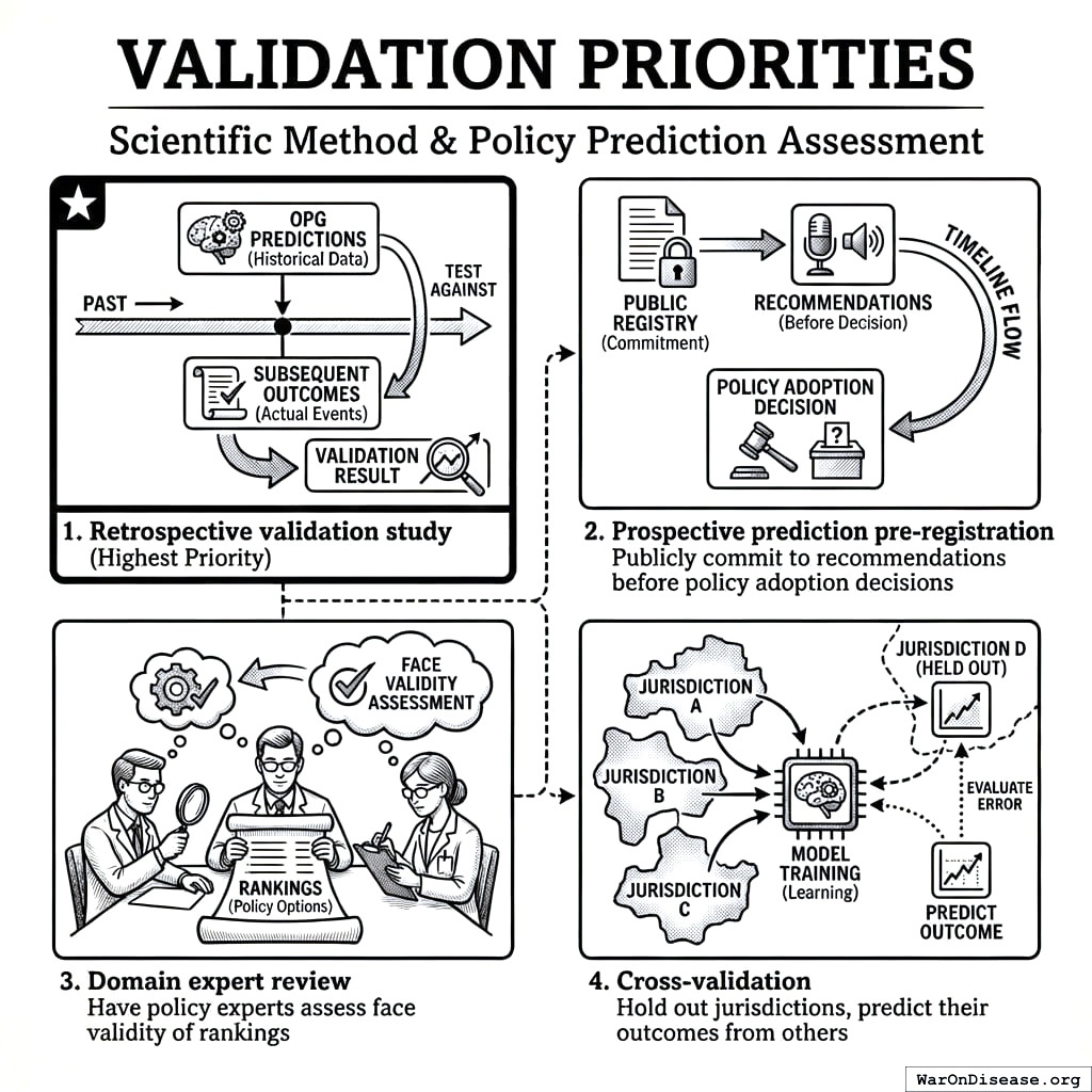
21.1 Validation Priorities
Ways to check if predictions work, ranked by importance: retrospective studies, prospective trials, cross-validation, expert review. Trust in descending order.
Retrospective validation study (highest priority): Test OPG predictions against subsequent outcomes
Prospective prediction pre-registration: Publicly commit to recommendations before policy adoption decisions
Domain expert review: Have policy experts assess face validity of rankings
Cross-validation: Hold out jurisdictions, predict their outcomes from others
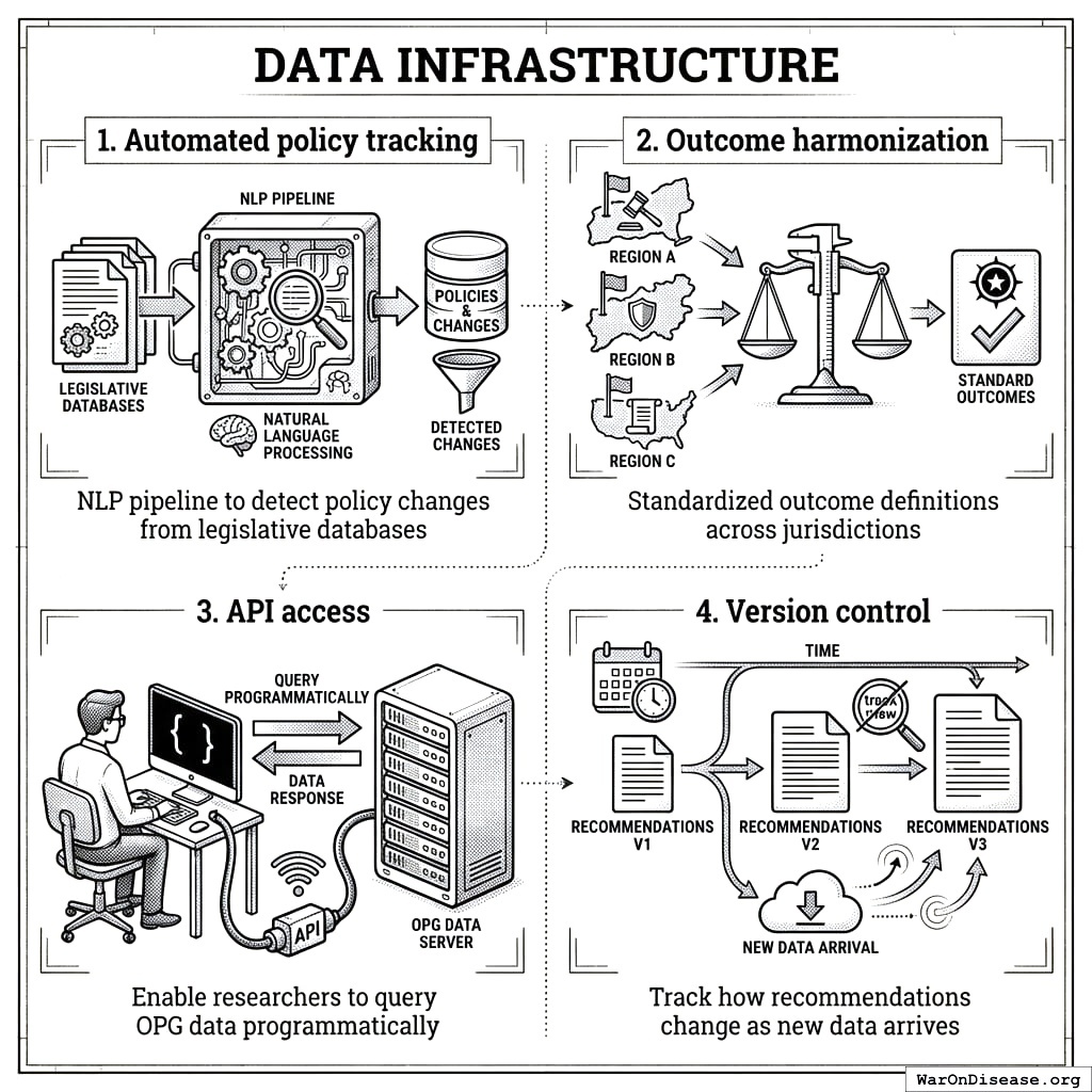
21.2 Data Infrastructure
Collect laws, teach computers to read them, standardize the results, give researchers access. It’s a library, but the books are alive and the librarian is an algorithm.
Automated policy tracking: NLP pipeline to detect policy changes from legislative databases
Outcome harmonization: Standardized outcome definitions across jurisdictions
API access: Enable researchers to query OPG data programmatically
Version control: Track how recommendations change as new data arrives
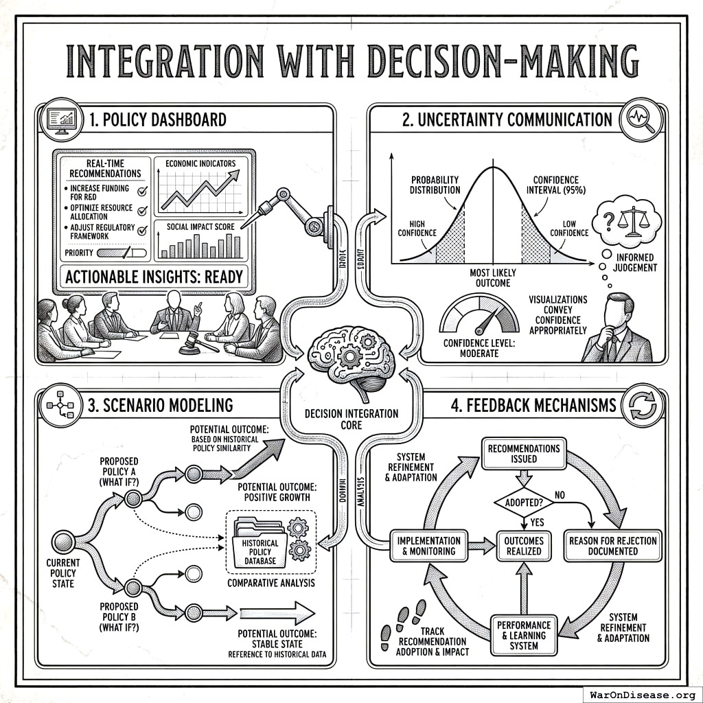
21.3 Integration with Decision-Making
Show data, admit uncertainty, model scenarios, get feedback, repeat. It’s like being honest about not knowing things, which is why it’s revolutionary.
Policy dashboard: Real-time recommendations for policymakers
Uncertainty communication: Visualizations that convey confidence appropriately
Scenario modeling: “What if” analysis for proposed policies based on similar historical policies
Feedback mechanisms: Track whether recommendations were actually adopted and outcomes realized
22 Conclusion
The Optimal Policy Generator provides a systematic framework for translating policy-outcome evidence into jurisdiction-specific recommendations. By comparing each jurisdiction’s current policy inventory to the evidence-supported set, OPG produces actionable recommendations in four categories (enact/replace/repeal/maintain) ranked by expected welfare impact. The framework transforms scattered natural experimental evidence into actionable, jurisdiction-specific guidance.
Acknowledgments
[To be added: acknowledgments for seminar participants, reviewers, and colleagues who provided feedback.]
23 References
1.
NIH Common Fund. NIH pragmatic trials: Minimal funding despite 30x cost advantage. NIH Common Fund: HCS Research Collaboratoryhttps://commonfund.nih.gov/hcscollaboratory (2025)
The NIH Pragmatic Trials Collaboratory funds trials at $500K for planning phase, $1M/year for implementation-a tiny fraction of NIH’s budget. The ADAPTABLE trial cost $14 million for 15,076 patients (= $929/patient) versus $420 million for a similar traditional RCT (30x cheaper), yet pragmatic trials remain severely underfunded. PCORnet infrastructure enables real-world trials embedded in healthcare systems, but receives minimal support compared to basic research funding. Additional sources: https://commonfund.nih.gov/hcscollaboratory | https://pcornet.org/wp-content/uploads/2025/08/ADAPTABLE_Lay_Summary_21JUL2025.pdf | https://www.ncbi.nlm.nih.gov/pmc/articles/PMC5604499/
Mean exclusion rate: 86.1% across 158 antidepressant efficacy trials (range: 44.4% to 99.8%) More than 82% of real-world depression patients would be ineligible for antidepressant registration trials Exclusion rates increased over time: 91.4% (2010-2014) vs. 83.8% (1995-2009) Most common exclusions: comorbid psychiatric disorders, age restrictions, insufficient depression severity, medical conditions Emergency psychiatry patients: only 3.3% eligible (96.7% excluded) when applying 9 common exclusion criteria Only a minority of depressed patients seen in clinical practice are likely to be eligible for most AETs Note: Generalizability of antidepressant trials has decreased over time, with increasingly stringent exclusion criteria eliminating patients who would actually use the drugs in clinical practice Additional sources: https://pubmed.ncbi.nlm.nih.gov/26276679/ | https://pubmed.ncbi.nlm.nih.gov/26164052/ | https://www.wolterskluwer.com/en/news/antidepressant-trials-exclude-most-real-world-patients-with-depression
Berkshire’s compounded annual return from 1965 through 2024 was 19.9%, nearly double the 10.4% recorded by the S&P 500. Berkshire shares skyrocketed 5,502,284% compared to the S&P 500’s 39,054% rise during that period. Additional sources: https://www.cnbc.com/2025/05/05/warren-buffetts-return-tally-after-60-years-5502284percent.html | https://www.slickcharts.com/berkshire-hathaway/returns
Comprehensive mortality and morbidity data by cause, age, sex, country, and year Global mortality: 55-60 million deaths annually Lives saved by modern medicine (vaccines, cardiovascular drugs, oncology): 12M annually (conservative aggregate) Leading causes of death: Cardiovascular disease (17.9M), Cancer (10.3M), Respiratory disease (4.0M) Note: Baseline data for regulatory mortality analysis. Conservative estimate of pharmaceutical impact based on WHO immunization data (4.5M/year from vaccines) + cardiovascular interventions (3.3M/year) + oncology (1.5M/year) + other therapies. Additional sources: https://www.who.int/data/gho/data/themes/mortality-and-global-health-estimates
General range: $3,000-$5,500 per life saved (GiveWell top charities) Helen Keller International (Vitamin A): $3,500 average (2022-2024); varies $1,000-$8,500 by country Against Malaria Foundation: $5,500 per life saved New Incentives (vaccination incentives): $4,500 per life saved Malaria Consortium (seasonal malaria chemoprevention): $3,500 per life saved VAS program details: $2 to provide vitamin A supplements to child for one year Note: Figures accurate for 2024. Helen Keller VAS program has wide country variation ($1K-$8.5K) but $3,500 is accurate average. Among most cost-effective interventions globally Additional sources: https://www.givewell.org/charities/top-charities | https://www.givewell.org/charities/helen-keller-international | https://ourworldindata.org/cost-effectiveness
Average family caregiver: 25-26 hours per week (100-104 hours per month) 38 million caregivers providing 36 billion hours of care annually Economic value: $16.59 per hour = $600 billion total annual value (2021) 28% of people provided eldercare on a given day, averaging 3.9 hours when providing care Caregivers living with care recipient: 37.4 hours per week Caregivers not living with recipient: 23.7 hours per week Note: Disease-related caregiving is subset of total; includes elderly care, disability care, and child care Additional sources: https://www.aarp.org/caregiving/financial-legal/info-2023/unpaid-caregivers-provide-billions-in-care.html | https://www.bls.gov/news.release/elcare.nr0.htm | https://www.caregiver.org/resource/caregiver-statistics-demographics/
US programs (1994-2023): $540B direct savings, $2.7T societal savings ( $18B/year direct, $90B/year societal) Global (2001-2020): $820B value for 10 diseases in 73 countries ( $41B/year) ROI: $11 return per $1 invested Measles vaccination alone saved 93.7M lives (61% of 154M total) over 50 years (1974-2024) Additional sources: https://www.cdc.gov/mmwr/volumes/73/wr/mm7331a2.htm | https://www.thelancet.com/journals/lancet/article/PIIS0140-6736(24)00850-X/fulltext
CPI-U (1980): 82.4 CPI-U (2024): 313.5 Inflation multiplier (1980-2024): 3.80× Cumulative inflation: 280.48% Average annual inflation rate: 3.08% Note: Official U.S. government inflation data using Consumer Price Index for All Urban Consumers (CPI-U). Additional sources: https://www.bls.gov/data/inflation_calculator.htm
.
10.
ClinicalTrials.gov API v2 direct analysis. ClinicalTrials.gov cumulative enrollment data (2025). Direct analysis via ClinicalTrials.gov API v2https://clinicaltrials.gov/data-api/api
Analysis of 100,000 active/recruiting/completed trials on ClinicalTrials.gov (as of January 2025) shows cumulative enrollment of 12.2 million participants: Phase 1 (722k), Phase 2 (2.2M), Phase 3 (6.5M), Phase 4 (2.7M). Median participants per trial: Phase 1 (33), Phase 2 (60), Phase 3 (237), Phase 4 (90). Additional sources: https://clinicaltrials.gov/data-api/api
Only 3-5% of adult cancer patients in US receive treatment within clinical trials About 5% of American adults have ever participated in any clinical trial Oncology: 2-3% of all oncology patients participate Contrast: 50-60% enrollment for pediatric cancer trials (<15 years old) Note: 20% of cancer trials fail due to insufficient enrollment; 11% of research sites enroll zero patients Additional sources: https://www.fightcancer.org/policy-resources/barriers-patient-enrollment-therapeutic-clinical-trials-cancer | https://hints.cancer.gov/docs/Briefs/HINTS_Brief_48.pdf
2.3 billion individuals had more than five ailments (2013) Chronic conditions caused 74% of all deaths worldwide (2019), up from 67% (2010) Approximately 1 in 3 adults suffer from multiple chronic conditions (MCCs) Risk factor exposures: 2B exposed to biomass fuel, 1B to air pollution, 1B smokers Projected economic cost: $47 trillion by 2030 Note: 2.3B with 5+ ailments is more accurate than "2B with chronic disease." One-third of all adults globally have multiple chronic conditions Additional sources: https://www.sciencedaily.com/releases/2015/06/150608081753.htm | https://pmc.ncbi.nlm.nih.gov/articles/PMC10830426/ | https://pmc.ncbi.nlm.nih.gov/articles/PMC6214883/
Approximately 12% of trials with results posted on the ClinicalTrials.gov results database (905/7,646) were terminated. Primary reasons: insufficient accrual (57% of non-data-driven terminations), business/strategic reasons, and efficacy/toxicity findings (21% data-driven terminations).
Global clinical trials market valued at approximately $83 billion in 2024, with projections to reach $83-132 billion by 2030. Additional sources: https://www.globenewswire.com/news-release/2024/04/19/2866012/0/en/Global-Clinical-Trials-Market-Research-Report-2024-An-83-16-Billion-Market-by-2030-AI-Machine-Learning-and-Blockchain-will-Transform-the-Clinical-Trials-Landscape.html | https://www.precedenceresearch.com/clinical-trials-market
Schistosomiasis treatment: $28.19-$70.48 per DALY (using arithmetic means with varying disability weights) Soil-transmitted helminths (STH) treatment: $82.54 per DALY (midpoint estimate) Note: GiveWell explicitly states this 2011 analysis is "out of date" and their current methodology focuses on long-term income effects rather than short-term health DALYs Additional sources: https://www.givewell.org/international/technical/programs/deworming/cost-effectiveness
.
19.
Calculated from IHME Global Burden of Disease (2.55B DALYs) and global GDP per capita valuation. $109 trillion annual global disease burden.
The global economic burden of disease, including direct healthcare costs ($8.2 trillion) and lost productivity ($100.9 trillion from 2.55 billion DALYs × $39,570 per DALY), totals approximately $109.1 trillion annually.
Phase I duration: 2.3 years average Total time to market (Phase I-III + approval): 10.5 years average Phase transition success rates: Phase I→II: 63.2%, Phase II→III: 30.7%, Phase III→Approval: 58.1% Overall probability of approval from Phase I: 12% Note: Largest publicly available study of clinical trial success rates. Efficacy lag = 10.5 - 2.3 = 8.2 years post-safety verification. Additional sources: https://go.bio.org/rs/490-EHZ-999/images/ClinicalDevelopmentSuccessRates2011_2020.pdf
Approximately 30% of drugs gain at least one new indication after initial approval. Additional sources: https://www.nature.com/articles/s41591-024-03233-x
Early childhood education: Benefits 12X outlays by 2050; $8.70 per dollar over lifetime Educational facilities: $1 spent → $1.50 economic returns Energy efficiency comparison: 2-to-1 benefit-to-cost ratio (McKinsey) Private return to schooling: 9% per additional year (World Bank meta-analysis) Note: 2.1 multiplier aligns with benefit-to-cost ratios for educational infrastructure/energy efficiency. Early childhood education shows much higher returns (12X by 2050) Additional sources: https://www.epi.org/publication/bp348-public-investments-outside-core-infrastructure/ | https://documents1.worldbank.org/curated/en/442521523465644318/pdf/WPS8402.pdf | https://freopp.org/whitepapers/establishing-a-practical-return-on-investment-framework-for-education-and-skills-development-to-expand-economic-opportunity/
Infrastructure fiscal multiplier: 1.6 during contractionary phase of economic cycle Average across all economic states: 1.5 (meaning $1 of public investment → $1.50 of economic activity) Time horizon: 0.8 within 1 year, 1.5 within 2-5 years Range of estimates: 1.5-2.0 (following 2008 financial crisis & American Recovery Act) Italian public construction: 1.5-1.9 multiplier US ARRA: 0.4-2.2 range (differential impacts by program type) Economic Policy Institute: Uses 1.6 for infrastructure spending (middle range of estimates) Note: Public investment less likely to crowd out private activity during recessions; particularly effective when monetary policy loose with near-zero rates Additional sources: https://blogs.worldbank.org/en/ppps/effectiveness-infrastructure-investment-fiscal-stimulus-what-weve-learned | https://www.gihub.org/infrastructure-monitor/insights/fiscal-multiplier-effect-of-infrastructure-investment/ | https://cepr.org/voxeu/columns/government-investment-and-fiscal-stimulus | https://www.richmondfed.org/publications/research/economic_brief/2022/eb_22-04
Ramey (2011): 0.6 short-run multiplier Barro (1981): 0.6 multiplier for WWII spending (war spending crowded out 40¢ private economic activity per federal dollar) Barro & Redlick (2011): 0.4 within current year, 0.6 over two years; increased govt spending reduces private-sector GDP portions General finding: $1 increase in deficit-financed federal military spending = less than $1 increase in GDP Variation by context: Central/Eastern European NATO: 0.6 on impact, 1.5-1.6 in years 2-3, gradual fall to zero Ramey & Zubairy (2018): Cumulative 1% GDP increase in military expenditure raises GDP by 0.7% Additional sources: https://www.mercatus.org/research/research-papers/defense-spending-and-economy | https://cepr.org/voxeu/columns/world-war-ii-america-spending-deficits-multipliers-and-sacrifice | https://www.rand.org/content/dam/rand/pubs/research_reports/RRA700/RRA739-2/RAND_RRA739-2.pdf
The FDA GRAS (Generally Recognized as Safe) list contains approximately 570–700 substances. Additional sources: https://www.fda.gov/food/generally-recognized-safe-gras/gras-notice-inventory
2024: 233,597 deaths (30% increase from 179,099 in 2023) Deadliest conflicts: Ukraine (67,000), Palestine (35,000) Nearly 200,000 acts of violence (25% higher than 2023, double from 5 years ago) One in six people globally live in conflict-affected areas Additional sources: https://acleddata.com/2024/12/12/data-shows-global-conflict-surged-in-2024-the-washington-post/ | https://acleddata.com/media-citation/data-shows-global-conflict-surged-2024-washington-post | https://acleddata.com/conflict-index/index-january-2024/
.
31.
UCDP. State violence deaths annually. UCDP: Uppsala Conflict Data Programhttps://ucdp.uu.se/
Uppsala Conflict Data Program (UCDP): Tracks one-sided violence (organized actors attacking unarmed civilians) UCDP definition: Conflicts causing at least 25 battle-related deaths in calendar year 2023 total organized violence: 154,000 deaths; Non-state conflicts: 20,900 deaths UCDP collects data on state-based conflicts, non-state conflicts, and one-sided violence Specific "2,700 annually" figure for state violence not found in recent UCDP data; actual figures vary annually Additional sources: https://ucdp.uu.se/ | https://en.wikipedia.org/wiki/Uppsala_Conflict_Data_Program | https://ourworldindata.org/grapher/deaths-in-armed-conflicts-by-region
2023: 8,352 deaths (22% increase from 2022, highest since 2017) 2023: 3,350 terrorist incidents (22% decrease), but 56% increase in avg deaths per attack Global Terrorism Database (GTD): 200,000+ terrorist attacks recorded (2021 version) Maintained by: National Consortium for Study of Terrorism & Responses to Terrorism (START), U. of Maryland Geographic shift: Epicenter moved from Middle East to Central Sahel (sub-Saharan Africa) - now >50% of all deaths Additional sources: https://ourworldindata.org/terrorism | https://reliefweb.int/report/world/global-terrorism-index-2024 | https://www.start.umd.edu/gtd/ | https://ourworldindata.org/grapher/fatalities-from-terrorism
.
33.
Institute for Health Metrics and Evaluation (IHME). IHME global burden of disease 2021 (2.88B DALYs, 1.13B YLD). Institute for Health Metrics and Evaluation (IHME)https://vizhub.healthdata.org/gbd-results/ (2024)
In 2021, global DALYs totaled approximately 2.88 billion, comprising 1.75 billion Years of Life Lost (YLL) and 1.13 billion Years Lived with Disability (YLD). This represents a 13% increase from 2019 (2.55B DALYs), largely attributable to COVID-19 deaths and aging populations. YLD accounts for approximately 39% of total DALYs, reflecting the substantial burden of non-fatal chronic conditions. Additional sources: https://vizhub.healthdata.org/gbd-results/ | https://www.thelancet.com/journals/lancet/article/PIIS0140-6736(24)00757-8/fulltext | https://www.healthdata.org/research-analysis/about-gbd
War on Terror emissions: 1.2B metric tons GHG (equivalent to 257M cars/year) Military: 5.5% of global GHG emissions (2X aviation + shipping combined) US DoD: World’s single largest institutional oil consumer, 47th largest emitter if nation Cleanup costs: $500B+ for military contaminated sites Gaza war environmental damage: $56.4B; landmine clearance: $34.6B expected Climate finance gap: Rich nations spend 30X more on military than climate finance Note: Military activities cause massive environmental damage through GHG emissions, toxic contamination, and long-term cleanup costs far exceeding current climate finance commitments Additional sources: https://watson.brown.edu/costsofwar/costs/social/environment | https://earth.org/environmental-costs-of-wars/ | https://transformdefence.org/transformdefence/stats/
Global military spending: $2.7 trillion (2024, SIPRI) Global government medical research: $68 billion (2024) Actual ratio: 39.7:1 in favor of weapons over medical research Military R&D alone: $85B (2004 data, 10% of global R&D) Military spending increases crowd out health: 1% ↑ military = 0.62% ↓ health spending Note: Ratio actually worse than 36:1. Each 1% increase in military spending reduces health spending by 0.62%, with effect more intense in poorer countries (0.962% reduction) Additional sources: https://www.sipri.org/commentary/blog/2016/opportunity-cost-world-military-spending | https://pmc.ncbi.nlm.nih.gov/articles/PMC9174441/ | https://www.congress.gov/crs-product/R45403
Lost human capital from war: $300B annually (economic impact of losing skilled/productive individuals to conflict) Broader conflict/violence cost: $14T/year globally 1.4M violent deaths/year; conflict holds back economic development, causes instability, widens inequality, erodes human capital 2002: 48.4M DALYs lost from 1.6M violence deaths = $151B economic value (2000 USD) Economic toll includes: commodity prices, inflation, supply chain disruption, declining output, lost human capital Additional sources: https://thinkbynumbers.org/military/war/the-economic-case-for-peace-a-comprehensive-financial-analysis/ | https://www.weforum.org/stories/2021/02/war-violence-costs-each-human-5-a-day/ | https://pubmed.ncbi.nlm.nih.gov/19115548/
PTSD economic burden (2018 U.S.): $232.2B total ($189.5B civilian, $42.7B military) Civilian costs driven by: Direct healthcare ($66B), unemployment ($42.7B) Military costs driven by: Disability ($17.8B), direct healthcare ($10.1B) Exceeds costs of other mental health conditions (anxiety, depression) War-exposed populations: 2-3X higher rates of anxiety, depression, PTSD; women and children most vulnerable Note: Actual burden $232B, significantly higher than "$100B" claimed Additional sources: https://pubmed.ncbi.nlm.nih.gov/35485933/ | https://news.va.gov/103611/study-national-economic-burden-of-ptsd-staggering/ | https://pmc.ncbi.nlm.nih.gov/articles/PMC9957523/
The average cost of supporting a refugee is $1,384 per year. This represents total host country costs (housing, healthcare, education, security). OECD countries average $6,100 per refugee (mean 2022-2023), with developing countries spending $700-1,000. Global weighted average of $1,384 is reasonable given that 75-85% of refugees are in low/middle-income countries. Additional sources: https://www.cgdev.org/blog/costs-hosting-refugees-oecd-countries-and-why-uk-outlier | https://www.unhcr.org/sites/default/files/2024-11/UNHCR-WB-global-cost-of-refugee-inclusion-in-host-country-health-systems.pdf
Estimated $616B annual cost from conflict-related trade disruption. World Bank research shows civil war costs an average developing country 30 years of GDP growth, with 20 years needed for trade to return to pre-war levels. Trade disputes analysis shows tariff escalation could reduce global exports by up to $674 billion. Additional sources: https://www.worldbank.org/en/topic/trade/publication/trading-away-from-conflict | https://www.nber.org/papers/w11565 | http://blogs.worldbank.org/en/trade/impacts-global-trade-and-income-current-trade-disputes
Global days of therapy reached 1.8 trillion in 2019 (234 defined daily doses per person). Diabetes, respiratory, CVD, and cancer account for 71 percent of medicine use. Projected to reach 3.8 trillion DDDs by 2028.
Estimated private pharmaceutical and biotech clinical trial spending is approximately $75-90 billion annually, representing roughly 90% of global clinical trial spending.
Quantifying the gap between current global governance and theoretical maximum welfare, estimating a 31-53% efficiency score and $97 trillion in annual opportunity costs.
Estimated range based on NIH ( $0.8-5.6B), NIHR ($1.6B total budget), and EU funding ( $1.3B/year). Roughly 5-10% of global market. Additional sources: https://www.appliedclinicaltrialsonline.com/view/sizing-clinical-research-market | https://www.thelancet.com/journals/langlo/article/PIIS2214-109X(20)30357-0/fulltext
Total global household wealth: USD 454.4 trillion (2022) Wealth declined by USD 11.3 trillion (-2.4%) in 2022, first decline since 2008 Wealth per adult: USD 84,718 Additional sources: https://www.ubs.com/global/en/family-office-uhnw/reports/global-wealth-report-2023.html
Estimated from major foundation budgets and activities. Nonprofit clinical trial funding estimate.
Nonprofit foundations spend an estimated $2-5 billion annually on clinical trials globally, representing approximately 2-5% of total clinical trial spending.
50.
Industry reports: IQVIA. Global pharmaceutical r&d spending.
Total global pharmaceutical R&D spending is approximately $300 billion annually. Clinical trials represent 15-20% of this total ($45-60B), with the remainder going to drug discovery, preclinical research, regulatory affairs, and manufacturing development.
Milestone: November 15, 2022 (UN World Population Prospects 2022) Day of Eight Billion" designated by UN Added 1 billion people in just 11 years (2011-2022) Growth rate: Slowest since 1950; fell under 1% in 2020 Future: 15 years to reach 9B (2037); projected peak 10.4B in 2080s Projections: 8.5B (2030), 9.7B (2050), 10.4B (2080-2100 plateau) Note: Milestone reached Nov 2022. Population growth slowing; will take longer to add next billion (15 years vs 11 years) Additional sources: https://www.un.org/en/desa/world-population-reach-8-billion-15-november-2022 | https://www.un.org/en/dayof8billion | https://en.wikipedia.org/wiki/Day_of_Eight_Billion
The research found that nonviolent campaigns were twice as likely to succeed as violent ones, and once 3.5% of the population were involved, they were always successful. Chenoweth and Maria Stephan studied the success rates of civil resistance efforts from 1900 to 2006, finding that nonviolent movements attracted, on average, four times as many participants as violent movements and were more likely to succeed. Key finding: Every campaign that mobilized at least 3.5% of the population in sustained protest was successful (in their 1900-2006 dataset) Note: The 3.5% figure is a descriptive statistic from historical analysis, not a guaranteed threshold. One exception (Bahrain 2011-2014 with 6%+ participation) has been identified. The rule applies to regime change, not policy change in democracies. Additional sources: https://www.hks.harvard.edu/centers/carr/publications/35-rule-how-small-minority-can-change-world | https://www.hks.harvard.edu/sites/default/files/2024-05/Erica%20Chenoweth_2020-005.pdf | https://www.bbc.com/future/article/20190513-it-only-takes-35-of-people-to-change-the-world | https://en.wikipedia.org/wiki/3.5%25_rule
Your DNA is 3 billion base pairs Read the entire code (Human Genome Project, completed 2003) Learned to edit it (CRISPR, discovered 2012) Additional sources: https://www.genome.gov/11006929/2003-release-international-consortium-completes-hgp | https://www.nobelprize.org/prizes/chemistry/2020/press-release/
Mapping 350,000+ clinical trials showed that only 12% of the human interactome has ever been targeted by drugs. Additional sources: https://pmc.ncbi.nlm.nih.gov/articles/PMC10749231/
The ICD-10 classification contains approximately 14,000 codes for diseases, signs and symptoms. Additional sources: https://icd.who.int/browse10/2019/en
Longevity escape velocity: Hypothetical point where medical advances extend life expectancy faster than time passes Term coined by Aubrey de Grey (biogerontologist) in 2004 paper; concept from David Gobel (Methuselah Foundation) Current progress: Science adds 3 months to lifespan per year; LEV requires adding >1 year per year Sinclair (Harvard): "There is no biological upper limit to age" - first person to live to 150 may already be born De Grey: 50% chance of reaching LEV by mid-to-late 2030s; SENS approach = damage repair rather than slowing damage Kurzweil (2024): LEV by 2029-2035, AI will simulate biological processes to accelerate solutions George Church: LEV "in a decade or two" via age-reversal clinical trials Natural lifespan cap: 120-150 years (Jeanne Calment record: 122); engineering approach could bypass via damage repair Key mechanisms: Epigenetic reprogramming, senolytic drugs, stem cell therapy, gene therapy, AI-driven drug discovery Current record: Jeanne Calment (122 years, 164 days) - record unbroken since 1997 Note: LEV is theoretical but increasingly plausible given demonstrated age reversal in mice (109% lifespan extension) and human cells (30-year epigenetic age reversal) Additional sources: https://en.wikipedia.org/wiki/Longevity_escape_velocity | https://pmc.ncbi.nlm.nih.gov/articles/PMC423155/ | https://www.popularmechanics.com/science/a36712084/can-science-cure-death-longevity/ | https://www.diamandis.com/blog/longevity-escape-velocity
Registered lobbyists: Over 12,000 (some estimates); 12,281 registered (2013) Former government employees as lobbyists: 2,200+ former federal employees (1998-2004), including 273 former White House staffers, 250 former Congress members & agency heads Congressional revolving door: 43% (86 of 198) lawmakers who left 1998-2004 became lobbyists; currently 59% leaving to private sector work for lobbying/consulting firms/trade groups Executive branch: 8% were registered lobbyists at some point before/after government service Additional sources: https://en.wikipedia.org/wiki/Lobbying_in_the_United_States | https://www.opensecrets.org/revolving-door | https://www.citizen.org/article/revolving-congress/ | https://www.propublica.org/article/we-found-a-staggering-281-lobbyists-whove-worked-in-the-trump-administration
Single measles vaccination: 167:1 benefit-cost ratio. MMR (measles-mumps-rubella) vaccination: 14:1 ROI. Historical US elimination efforts (1966-1974): benefit-cost ratio of 10.3:1 with net benefits exceeding USD 1.1 billion (1972 dollars, or USD 8.0 billion in 2023 dollars). 2-dose MMR programs show direct benefit/cost ratio of 14.2 with net savings of $5.3 billion, and 26.0 from societal perspectives with net savings of $11.6 billion. Additional sources: https://www.mdpi.com/2076-393X/12/11/1210 | https://www.tandfonline.com/doi/full/10.1080/14760584.2024.2367451
One in four people in the world will be affected by mental or neurological disorders at some point in their lives, representing [approximately] 30% of the global burden of disease. Additional sources: https://www.who.int/news/item/28-09-2001-the-world-health-report-2001-mental-disorders-affect-one-in-four-people
Under the current system, approximately 10-15 diseases per year receive their FIRST effective treatment. Calculation: 5% of 7,000 rare diseases ( 350) have FDA-approved treatment, accumulated over 40 years of the Orphan Drug Act = 9 rare diseases/year. Adding 5-10 non-rare diseases that get first treatments yields 10-20 total. FDA approves 50 drugs/year, but many are for diseases that already have treatments (me-too drugs, second-line therapies). Only 15 represent truly FIRST treatments for previously untreatable conditions.
The budget total of $47.7 billion also includes $1.412 billion derived from PHS Evaluation financing... Additional sources: https://www.nih.gov/about-nih/organization/budget | https://officeofbudget.od.nih.gov/
Typical cost-effectiveness thresholds for medical interventions in rich countries range from $50,000 to $150,000 per QALY. The Institute for Clinical and Economic Review (ICER) uses a $100,000-$150,000/QALY threshold for value-based pricing. Between 1990-2021, authors increasingly cited $100,000 (47% by 2020-21) or $150,000 (24% by 2020-21) per QALY as benchmarks for cost-effectiveness. Additional sources: https://pmc.ncbi.nlm.nih.gov/articles/PMC10114019/ | https://icer.org/our-approach/methods-process/cost-effectiveness-the-qaly-and-the-evlyg/
Recent surveys: 49-51% willingness (2020-2022) - dramatic drop from 85% (2019) during COVID-19 pandemic Cancer patients when approached: 88% consented to trials (Royal Marsden Hospital) Study type variation: 44.8% willing for drug trial, 76.2% for diagnostic study Top motivation: "Learning more about my health/medical condition" (67.4%) Top barrier: "Worry about experiencing side effects" (52.6%) Additional sources: https://trialsjournal.biomedcentral.com/articles/10.1186/s13063-015-1105-3 | https://www.appliedclinicaltrialsonline.com/view/industry-forced-to-rethink-patient-participation-in-trials | https://pmc.ncbi.nlm.nih.gov/articles/PMC7183682/
.
68.
Tufts CSDD. Cost of drug development.
Various estimates suggest $1.0 - $2.5 billion to bring a new drug from discovery through FDA approval, spread across 10 years. Tufts Center for the Study of Drug Development often cited for $1.0 - $2.6 billion/drug. Industry reports (IQVIA, Deloitte) also highlight $2+ billion figures.
Study of 361 FDA-approved drugs from 1995-2014 (median follow-up 13.2 years): Mean lifetime revenue: $15.2 billion per drug Median lifetime revenue: $6.7 billion per drug Revenue after 5 years: $3.2 billion (mean) Revenue after 10 years: $9.5 billion (mean) Revenue after 15 years: $19.2 billion (mean) Distribution highly skewed: top 25 drugs (7%) accounted for 38% of total revenue ($2.1T of $5.5T) Additional sources: https://www.sciencedirect.com/science/article/pii/S1098301524027542
Using 3-way fixed-effects methodology (disease-country-year) across 66 diseases in 22 countries, this study estimates that drugs launched after 1981 saved 148.7 million life-years in 2013 alone. The regression coefficients for drug launches 0-11 years prior (beta=-0.031, SE=0.008) and 12+ years prior (beta=-0.057, SE=0.013) on years of life lost are highly significant (p<0.0001). Confidence interval for life-years saved: 79.4M-239.8M (95 percent CI) based on propagated standard errors from Table 2.
Deloitte’s annual study of top 20 pharma companies by R&D spend (2010-2024): 2024 ROI: 5.9% (second year of growth after decade of decline) 2023 ROI: 4.3% (estimated from trend) 2022 ROI: 1.2% (historic low since study began, 13-year low) 2021 ROI: 6.8% (record high, inflated by COVID-19 vaccines/treatments) Long-term trend: Declining for over a decade before 2023 recovery Average R&D cost per asset: $2.3B (2022), $2.23B (2024) These returns (1.2-5.9% range) fall far below typical corporate ROI targets (15-20%) Additional sources: https://www.deloitte.com/ch/en/Industries/life-sciences-health-care/research/measuring-return-from-pharmaceutical-innovation.html | https://www.prnewswire.com/news-releases/deloittes-13th-annual-pharmaceutical-innovation-report-pharma-rd-return-on-investment-falls-in-post-pandemic-market-301738807.html | https://hitconsultant.net/2023/02/16/pharma-rd-roi-falls-to-lowest-level-in-13-years/
.
72.
Nature Reviews Drug Discovery. Drug trial success rate from phase i to approval. Nature Reviews Drug Discovery: Clinical Success Rateshttps://www.nature.com/articles/nrd.2016.136 (2016)
Overall Phase I to approval: 10-12.8% (conventional wisdom 10%, studies show 12.8%) Recent decline: Average LOA now 6.7% for Phase I (2014-2023 data) Leading pharma companies: 14.3% average LOA (range 8-23%) Varies by therapeutic area: Oncology 3.4%, CNS/cardiovascular lowest at Phase III Phase-specific success: Phase I 47-54%, Phase II 28-34%, Phase III 55-70% Note: 12% figure accurate for historical average. Recent data shows decline to 6.7%, with Phase II as primary attrition point (28% success) Additional sources: https://www.nature.com/articles/nrd.2016.136 | https://pmc.ncbi.nlm.nih.gov/articles/PMC6409418/ | https://academic.oup.com/biostatistics/article/20/2/273/4817524
Phase 3 clinical trials cost between $20 million and $282 million per trial, with significant variation by therapeutic area and trial complexity. Additional sources: https://www.sofpromed.com/how-much-does-a-clinical-trial-cost | https://www.cbo.gov/publication/57126
Meta-analysis of 108 embedded pragmatic clinical trials (2006-2016). The median cost per patient was $97 (IQR $19–$478), based on 2015 dollars. 25% of trials cost <$19/patient; 10 trials exceeded $1,000/patient. U.S. studies median $187 vs non-U.S. median $27. Additional sources: https://pmc.ncbi.nlm.nih.gov/articles/PMC6508852/
For every dollar spent, the return on investment is nearly US$ 39." Total investment cost of US$ 7.5 billion generates projected economic and social benefits of US$ 289.2 billion from sustaining polio assets and integrating them into expanded immunization, surveillance and emergency response programmes across 8 priority countries (Afghanistan, Iraq, Libya, Pakistan, Somalia, Sudan, Syria, Yemen). Additional sources: https://www.who.int/news-room/feature-stories/detail/sustaining-polio-investments-offers-a-high-return
ICBL: Founded 1992 by 6 NGOs (Handicap International, Human Rights Watch, Medico International, Mines Advisory Group, Physicians for Human Rights, Vietnam Veterans of America Foundation) Started with ONE staff member: Jody Williams as founding coordinator Grew to 1,000+ organizations in 60 countries by 1997 Ottawa Process: 14 months (October 1996 - December 1997) Convention signed by 122 states on December 3, 1997; entered into force March 1, 1999 Achievement: Nobel Peace Prize 1997 (shared by ICBL and Jody Williams) Government funding context: Canada established $100M CAD Canadian Landmine Fund over 10 years (1997); International donors provided $169M in 1997 for mine action (up from $100M in 1996) Additional sources: https://www.icrc.org/en/doc/resources/documents/article/other/57jpjn.htm | https://en.wikipedia.org/wiki/International_Campaign_to_Ban_Landmines | https://www.nobelprize.org/prizes/peace/1997/summary/ | https://un.org/press/en/1999/19990520.MINES.BRF.html | https://www.the-monitor.org/en-gb/reports/2003/landmine-monitor-2003/mine-action-funding.aspx
388 former members of Congress are registered as lobbyists. Nearly 5,400 former congressional staffers have left Capitol Hill to become federal lobbyists in the past 10 years. Additional sources: https://www.opensecrets.org/revolving-door
Research identified 1,600+ medicines available in 1962. The 1950s represented industry high-water mark with >30 new products in five of ten years; this rate would not be replicated until late 1990s. More than half (880) of these medicines were lost following implementation of Kefauver-Harris Amendment. The peak of 1962 would not be seen again until early 21st century. By 2016 number of organizations actively involved in R&D at level not seen since 1914.
Pre-1962: Average cost per new chemical entity (NCE) was $6.5 million (1980 dollars) Inflation-adjusted to 2024 dollars: $6.5M (1980) ≈ $22.5M (2024), using CPI multiplier of 3.46× Real cost increase (inflation-adjusted): $22.5M (pre-1962) → $2,600M (2024) = 116× increase Note: This represents the most comprehensive academic estimate of pre-1962 drug development costs based on empirical industry data Additional sources: https://samizdathealth.org/wp-content/uploads/2020/12/hlthaff.1.2.6.pdf
Pre-1962: Physicians could report real-world evidence directly 1962 Drug Amendments replaced "premarket notification" with "premarket approval", requiring extensive efficacy testing Impact: New regulatory clampdown reduced new treatment production by 70%; lifespan growth declined from 4 years/decade to 2 years/decade Drug Efficacy Study Implementation (DESI): NAS/NRC evaluated 3,400+ drugs approved 1938-1962 for safety only; reviewed >3,000 products, >16,000 therapeutic claims FDA has had authority to accept real-world evidence since 1962, clarified by 21st Century Cures Act (2016) Note: Specific "144,000 physicians" figure not verified in sources Additional sources: https://thinkbynumbers.org/health/how-many-net-lives-does-the-fda-save/ | https://www.fda.gov/drugs/enforcement-activities-fda/drug-efficacy-study-implementation-desi | http://www.nasonline.org/about-nas/history/archives/collections/des-1966-1969-1.html
The RECOVERY trial, for example, cost only about $500 per patient... By contrast, the median per-patient cost of a pivotal trial for a new therapeutic is around $41,000. Additional sources: https://manhattan.institute/article/slow-costly-clinical-trials-drag-down-biomedical-breakthroughs
Dexamethasone saved 1 million lives worldwide (NHS England estimate, March 2021, 9 months after discovery). UK alone: 22,000 lives saved. Methodology: Águas et al. Nature Communications 2021 estimated 650,000 lives (range: 240,000-1,400,000) for July-December 2020 alone, based on RECOVERY trial mortality reductions (36% for ventilated, 18% for oxygen-only patients) applied to global COVID hospitalizations. June 2020 announcement: Dexamethasone reduced deaths by up to 1/3 (ventilated patients), 1/5 (oxygen patients). Impact immediate: Adopted into standard care globally within hours of announcement. Additional sources: https://www.england.nhs.uk/2021/03/covid-treatment-developed-in-the-nhs-saves-a-million-lives/ | https://www.nature.com/articles/s41467-021-21134-2 | https://pharmaceutical-journal.com/article/news/steroid-has-saved-the-lives-of-one-million-covid-19-patients-worldwide-figures-show | https://www.recoverytrial.net/news/recovery-trial-celebrates-two-year-anniversary-of-life-saving-dexamethasone-result
2,977 people were killed in the September 11, 2001 attacks: 2,753 at the World Trade Center, 184 at the Pentagon, and 40 passengers and crew on United Flight 93 in Shanksville, Pennsylvania.
Singapore GDP per capita (2023): $82,000 - among highest in the world Government spending: 15% of GDP (vs US 38%) Life expectancy: 84.1 years (vs US 77.5 years) Singapore demonstrates that low government spending can coexist with excellent outcomes Additional sources: https://data.worldbank.org/country/singapore
Singapore government spending is approximately 15% of GDP This is 23 percentage points lower than the United States (38%) Despite lower spending, Singapore achieves excellent outcomes: - Life expectancy: 84.1 years (vs US 77.5) - Low crime, world-class infrastructure, AAA credit rating Additional sources: https://www.imf.org/en/Countries/SGP
Life expectancy at birth varies significantly among developed nations: Switzerland: 84.0 years (2023) Singapore: 84.1 years (2023) Japan: 84.3 years (2023) United States: 77.5 years (2023) - 6.5 years below Switzerland, Singapore Global average: 73 years Note: US spends more per capita on healthcare than any other nation, yet achieves lower life expectancy Additional sources: https://www.who.int/data/gho/data/themes/mortality-and-global-health-estimates/ghe-life-expectancy-and-healthy-life-expectancy
Population-level: Up to 14% (9% men, 14% women) of total life expectancy gain since 1960 due to tobacco control efforts Individual cessation benefits: Quitting at age 35 adds 6.9-8.5 years (men), 6.1-7.7 years (women) vs continuing smokers By cessation age: Age 25-34 = 10 years gained; age 35-44 = 9 years; age 45-54 = 6 years; age 65 = 2.0 years (men), 3.7 years (women) Cessation before age 40: Reduces death risk by 90% Long-term cessation: 10+ years yields survival comparable to never smokers, averts 10 years of life lost Recent cessation: <3 years averts 5 years of life lost Additional sources: https://www.ncbi.nlm.nih.gov/pmc/articles/PMC1447499/ | https://www.cdc.gov/pcd/issues/2012/11_0295.htm | https://www.ajpmonline.org/article/S0749-3797(24)00217-4/fulltext | https://www.nejm.org/doi/full/10.1056/NEJMsa1211128
Standard economic value per QALY: $100,000–$150,000. This is the US and global standard willingness-to-pay threshold for interventions that add costs. Dominant interventions (those that save money while improving health) are favorable regardless of this threshold. Additional sources: https://icer.org/wp-content/uploads/2024/02/Reference-Case-4.3.25.pdf
Consumer costs: $2.5-3.5 billion per year (GAO estimate) Net economic cost: $1 billion per year 2022: US consumers paid 2X world price for sugar Program costs $3-4 billion/year but no federal budget impact (costs passed directly to consumers via higher prices) Employment impact: 10,000-20,000 manufacturing jobs lost annually in sugar-reliant industries (confectionery, etc.) Multiple studies confirm: Sweetener Users Association ($2.9-3.5B), AEI ($2.4B consumer cost), Beghin & Elobeid ($2.9-3.5B consumer surplus) Additional sources: https://www.gao.gov/products/gao-24-106144 | https://www.heritage.org/agriculture/report/the-us-sugar-program-bad-consumers-bad-agriculture-and-bad-america | https://www.aei.org/articles/the-u-s-spends-4-billion-a-year-subsidizing-stalinist-style-domestic-sugar-production/
2023: 0.70272% of GDP (World Bank) 2024: CHF 5.95 billion official military spending When including militia system costs: 1% GDP (CHF 8.75B) Comparison: Near bottom in Europe; only Ireland, Malta, Moldova spend less (excluding microstates with no armies) Additional sources: https://data.worldbank.org/indicator/MS.MIL.XPND.GD.ZS?locations=CH | https://www.avenir-suisse.ch/en/blog-defence-spending-switzerland-is-in-better-shape-than-it-seems/ | https://tradingeconomics.com/switzerland/military-expenditure-percent-of-gdp-wb-data.html
2024 GDP per capita (PPP-adjusted): Switzerland $93,819 vs United States $75,492 Switzerland’s GDP per capita 24% higher than US when adjusted for purchasing power parity Nominal 2024: Switzerland $103,670 vs US $85,810 Additional sources: https://data.worldbank.org/indicator/NY.GDP.PCAP.CD?locations=CH | https://tradingeconomics.com/switzerland/gdp-per-capita-ppp | https://www.theglobaleconomy.com/USA/gdp_per_capita_ppp/
OECD government spending data shows significant variation among developed nations: United States: 38.0% of GDP (2023) Switzerland: 35.0% of GDP - 3 percentage points lower than US Singapore: 15.0% of GDP - 23 percentage points lower than US (per IMF data) OECD average: approximately 40% of GDP Additional sources: https://data.oecd.org/gga/general-government-spending.htm
Chance of American dying in foreign-born terrorist attack: 1 in 3.6 million per year (1975-2015) Including 9/11 deaths; annual murder rate is 253x higher than terrorism death rate More likely to die from lightning strike than foreign terrorism Note: Comprehensive 41-year study shows terrorism risk is extremely low compared to everyday dangers Additional sources: https://www.cato.org/policy-analysis/terrorism-immigration-risk-analysis | https://www.nbcnews.com/news/us-news/you-re-more-likely-die-choking-be-killed-foreign-terrorists-n715141
The total number of embryos affected by the use of thalidomide during pregnancy is estimated at 10,000, of whom about 40% died around the time of birth. More than 10,000 children in 46 countries were born with deformities such as phocomelia. Additional sources: https://en.wikipedia.org/wiki/Thalidomide_scandal
Study of thalidomide survivors documenting ongoing disability impacts, quality of life, and long-term health outcomes. Survivors (now in their 60s) continue to experience significant disability from limb deformities, organ damage, and other effects. Additional sources: https://journals.plos.org/plosone/article?id=10.1371/journal.pone.0210222
US Census Bureau historical estimates of world population by country and region (1950-2050). US population in 1960: 180 million of 3 billion worldwide (6%). Additional sources: https://www.census.gov/data/tables/time-series/demo/international-programs/historical-est-worldpop.html
Overall, the 138 clinical trials had an estimated median (IQR) cost of $19.0 million ($12.2 million-$33.1 million)... The clinical trials cost a median (IQR) of $41,117 ($31,802-$82,362) per patient. Additional sources: https://www.ncbi.nlm.nih.gov/pmc/articles/PMC6248200/
Disability weights for 235 health states used in Global Burden of Disease calculations. Weights range from 0 (perfect health) to 1 (death equivalent). Chronic conditions like diabetes (0.05-0.35), COPD (0.04-0.41), depression (0.15-0.66), and cardiovascular disease (0.04-0.57) show substantial variation by severity. Treatment typically reduces disability weights by 50-80 percent for manageable chronic conditions.
Chronic diseases account for 90% of U.S. healthcare spending ( $3.7T/year). Additional sources: https://www.cdc.gov/chronic-disease/data-research/facts-stats/index.html
US GDP reached $28.78 trillion in 2024, representing approximately 26% of global GDP. Additional sources: https://data.worldbank.org/indicator/NY.GDP.MKTP.CD?locations=US | https://www.bea.gov/news/2024/gross-domestic-product-fourth-quarter-and-year-2024-advance-estimate
.
108.
Environmental Working Group. US farm subsidy database and analysis. Environmental Working Grouphttps://farm.ewg.org/ (2024)
US agricultural subsidies total approximately $30 billion annually, but create much larger economic distortions. Top 10% of farms receive 78% of subsidies, benefits concentrated in commodity crops (corn, soy, wheat, cotton), environmental damage from monoculture incentivized, and overall deadweight loss estimated at $50-120 billion annually. Additional sources: https://farm.ewg.org/ | https://www.ers.usda.gov/topics/farm-economy/farm-sector-income-finances/government-payments-the-safety-net/
Since 1971, the war on drugs has cost the United States an estimated $1 trillion in enforcement. The federal drug control budget was $41 billion in 2022. Mass incarceration costs the U.S. at least $182 billion every year, with over $450 billion spent to incarcerate individuals on drug charges in federal prisons.
Globally, fossil fuel subsidies were $7 trillion in 2022 or 7.1 percent of GDP. The United States subsidies totaled $649 billion. Underpricing for local air pollution costs and climate damages are the largest contributor, accounting for about 30 percent each.
The US spent approximately twice as much as other high-income countries on medical care (mean per capita: $9,892 vs $5,289), with similar utilization but much higher prices. Administrative costs accounted for 8% of US spending vs 1-3% in other countries. US spending on pharmaceuticals was $1,443 per capita vs $749 elsewhere. Despite spending more, US health outcomes are not better. Additional sources: https://jamanetwork.com/journals/jama/article-abstract/2674671
We quantify the amount of spatial misallocation of labor across US cities and its aggregate costs. Tight land-use restrictions in high-productivity cities like New York, San Francisco, and Boston lowered aggregate US growth by 36% from 1964 to 2009. Local constraints on housing supply have had enormous effects on the national economy. Additional sources: https://www.aeaweb.org/articles?id=10.1257/mac.20170388
Accounting for all the 2025 US tariffs and retaliation implemented to date, the level of real GDP is persistently -0.6% smaller in the long run, the equivalent of $160 billion 2024$ annually.
Americans will spend over 7.9 billion hours complying with IRS tax filing and reporting requirements in 2024. This costs the economy roughly $413 billion in lost productivity. In addition, the IRS estimates that Americans spend roughly $133 billion annually in out-of-pocket costs, bringing the total compliance costs to $546 billion, or nearly 2 percent of GDP.
Heart failure alone: $108 billion/year (2012 global analysis, 197 countries) US CVD: $555B (2016) → projected $1.8T by 2050 LMICs total CVD loss: $3.7T cumulative (2011-2015, 5-year period) CVD is costliest disease category in most developed nations Note: No single $2.1T global figure found; estimates vary widely by scope and year Additional sources: https://www.ahajournals.org/doi/10.1161/CIR.0000000000001258
US life expectancy at birth was 77.5 years in 2023 Male life expectancy: 74.8 years Female life expectancy: 80.2 years This is 6-7 years lower than peer developed nations despite higher healthcare spending Additional sources: https://www.cdc.gov/nchs/fastats/life-expectancy.htm
US median household income was $77,500 in 2023 Real median household income declined 0.8% from 2022 Gini index: 0.467 (income inequality measure) Additional sources: https://www.census.gov/library/publications/2024/demo/p60-282.html
US military spending in constant 2024 dollars: 1939 $29B (pre-WW2 baseline), 1940 $37B, 1944 $1,383B, 1945 $1,420B (peak), 1946 $674B, 1947 $176B, 1948 $117B, 2024 $886B. The post-WW2 demobilization cut spending 88% in two years (1945-1947). Current peacetime spending ($886B) is 30x the pre-WW2 baseline and 62% of peak WW2 spending, in inflation-adjusted dollars.
U.S. military spending amounted to 3.5% of GDP in 2024. In 2024, the U.S. spent nearly $1 trillion on its military budget, equal to 3.4% of GDP. Additional sources: https://www.statista.com/statistics/262742/countries-with-the-highest-military-spending/ | https://www.sipri.org/sites/default/files/2025-04/2504_fs_milex_2024.pdf
73.6% (or 174 million people) of the citizen voting-age population was registered to vote in 2024 (Census Bureau). More than 211 million citizens were active registered voters (86.6% of citizen voting age population) according to the Election Assistance Commission. Additional sources: https://www.census.gov/newsroom/press-releases/2025/2024-presidential-election-voting-registration-tables.html | https://www.eac.gov/news/2025/06/30/us-election-assistance-commission-releases-2024-election-administration-and-voting
The Constitution provides that the president ’shall have Power, by and with the Advice and Consent of the Senate, to make Treaties, provided two-thirds of the Senators present concur’ (Article II, section 2). Treaties are formal agreements with foreign nations that require two-thirds Senate approval. 67 senators (two-thirds of 100) must vote to ratify a treaty for it to take effect. Additional sources: https://www.senate.gov/about/powers-procedures/treaties.htm
Presidential candidates raised $2 billion; House and Senate candidates raised $3.8 billion and spent $3.7 billion; PACs raised $15.7 billion and spent $15.5 billion. Total federal campaign spending approximately $20 billion. Additional sources: https://www.fec.gov/updates/statistical-summary-of-24-month-campaign-activity-of-the-2023-2024-election-cycle/
Total federal lobbying reached record $4.4 billion in 2024. The $150 million increase in lobbying continues an upward trend that began in 2016. Additional sources: https://www.opensecrets.org/news/2025/02/federal-lobbying-set-new-record-in-2024/
National average: 1 in 60 million chance (2008 election analysis by Gelman, Silver, Edlin) Swing states (NM, VA, NH, CO): 1 in 10 million chance Non-competitive states: 34 states >1 in 100 million odds; 20 states >1 in 1 billion Washington DC: 1 in 490 billion odds Methodology: Probability state is necessary for electoral college win × probability state vote is tied Additional sources: https://sites.stat.columbia.edu/gelman/research/published/probdecisive2.pdf | https://onlinelibrary.wiley.com/doi/abs/10.1111/j.1465-7295.2010.00272.x
The overall failure rate of drugs that passed into Phase 1 trials to final approval is 90%. This lack of translation from promising preclinical findings to success in human trials is known as the "valley of death." Estimated 30-50% of promising compounds never proceed to Phase 2/3 trials primarily due to funding barriers rather than scientific failure. The late-stage attrition rate for oncology drugs is as high as 70% in Phase II and 59% in Phase III trials.
Current VSL (2024): $13.7 million (updated from $13.6M) Used in cost-benefit analyses for transportation regulations and infrastructure Methodology updated in 2013 guidance, adjusted annually for inflation and real income VSL represents aggregate willingness to pay for safety improvements that reduce fatalities by one Note: DOT has published VSL guidance periodically since 1993. Current $13.7M reflects 2024 inflation/income adjustments Additional sources: https://www.transportation.gov/office-policy/transportation-policy/revised-departmental-guidance-on-valuation-of-a-statistical-life-in-economic-analysis | https://www.transportation.gov/regulations/economic-values-used-in-analysis
India: $23-$50 per DALY averted (least costly intervention, $1,000-$6,100 per death averted) Sub-Saharan Africa (2022): $220-$860 per DALY (Burkina Faso: $220, Kenya: $550, Nigeria: $860) WHO estimates for Africa: $40 per DALY for fortification, $255 for supplementation Uganda fortification: $18-$82 per DALY (oil: $18, sugar: $82) Note: Wide variation reflects differences in baseline VAD prevalence, coverage levels, and whether intervention is supplementation or fortification Additional sources: https://journals.plos.org/plosone/article?id=10.1371/journal.pone.0012046 | https://journals.plos.org/plosone/article?id=10.1371/journal.pone.0266495
The $50,000/QALY threshold is widely used in US health economics literature, originating from dialysis cost benchmarks in the 1980s. In US cost-utility analyses, 77.5% of authors use either $50,000 or $100,000 per QALY as reference points. Most successful health programs cost $3,000-10,000 per QALY. WHO-CHOICE uses GDP per capita multiples (1× GDP/capita = "very cost-effective", 3× GDP/capita = "cost-effective"), which for the US ( $70,000 GDP/capita) translates to $70,000-$210,000/QALY thresholds. Additional sources: https://pmc.ncbi.nlm.nih.gov/articles/PMC5193154/ | https://pmc.ncbi.nlm.nih.gov/articles/PMC9278384/
78.4% of U.S. employees have at least one chronic condition (7% increase since 2021) 58% of employees report physical chronic health conditions 28% of all employees experience productivity loss due to chronic conditions Average productivity loss: $4,798 per employee per year Employees with 3+ chronic conditions miss 7.8 days annually vs 2.2 days for those without Note: 28% productivity loss translates to roughly 11 hours per week (28% of 40-hour workweek) Additional sources: https://www.ibiweb.org/resources/chronic-conditions-in-the-us-workforce-prevalence-trends-and-productivity-impacts | https://www.onemedical.com/mediacenter/study-finds-more-than-half-of-employees-are-living-with-chronic-conditions-including-1-in-3-gen-z-and-millennial-employees/ | https://debeaumont.org/news/2025/poll-the-toll-of-chronic-health-conditions-on-employees-and-workplaces/
Smokers lose at least one decade of life expectancy compared with those who have never smoked. The probability of surviving from 25 to 79 years of age was about twice as great in those who had never smoked as in current smokers (70 percent vs. 38 percent among women and 61 percent vs. 26 percent among men). Cessation before age 40 reduces the risk of death associated with continued smoking by about 90 percent. Adults who quit at ages 25-34, 35-44, or 45-54 gained about 10, 9, and 6 years of life respectively compared with those who continued to smoke.
134.
Blincoe, L. J., Miller, T. R., Zaloshnja, E. & Lawrence, B. A. The Economic and Societal Impact of Motor Vehicle Crashes, 2010 (Revised). https://rosap.ntl.bts.gov/view/dot/78697 (2015)
In 2010, there were 32,999 people killed, 3.9 million injured, and 24 million vehicles damaged in motor vehicle crashes in the United States. The economic costs totaled \(277 billion. When quality of life valuations are considered, the total value of societal harm from motor vehicle crashes was\)871 billion, representing 1.9 percent of GDP.
135.
Buchanan, J. M. & Tullock, G. The Calculus of Consent: Logical Foundations of Constitutional Democracy. (University of Michigan Press, Ann Arbor, 1962).
136.
Olson, M. The Logic of Collective Action: Public Goods and the Theory of Groups. (Harvard University Press, Cambridge, MA, 1965).
137.
Stigler, G. J. The theory of economic regulation. Stigler2, 3–21 (1971)
As a rule, regulation is acquired by the industry and is designed and operated primarily for its benefit.
138.
Becker, G. S. A theory of competition among pressure groups for political influence. Becker98, 371–400 (1983)
Political equilibrium depends on the efficiency of each group in producing pressure, the effect of additional pressure on their influence, the number of persons in different groups, and the deadweight cost of taxes and subsidies.
139.
Cartwright, N. & Hardie, J. Evidence-Based Policy: A Practical Guide to Doing It Better. (Cartwright, Oxford, 2012).
The key to evidence-based policy is understanding that evidence of effectiveness elsewhere is not evidence of effectiveness here without support for the claim that the causal mechanism will operate in the new setting.
140.
Haskins, R. & Margolis, G. Show Me the Evidence: Obama’s Fight for Rigor and Results in Social Policy. (Haskins, Washington, DC, 2009).
The federal government spends hundreds of billions of dollars annually on social programs with little rigorous evidence of effectiveness.
141.
Hahn, R. W. Regulatory reform: What do the government’s numbers tell us? in 208–253 (2000).
A review of 48 regulatory impact analyses finds substantial variation in methodology and quality, with many failing to provide adequate justification for regulatory choices.
The WWC reviews existing research on different programs, products, practices, and policies in education to provide educators with the information they need to make evidence-based decisions.
Heterogeneity in systematic reviews refers to variability among studies. I² describes the percentage of variability in effect estimates that is due to heterogeneity rather than sampling error.
144.
Petticrew, M. & Roberts, H. Systematic Reviews in the Social Sciences: A Practical Guide. (Petticrew, Malden, MA, 2006).
Systematic reviews can help policymakers by providing a rigorous and transparent method for synthesizing research evidence on the effectiveness of social interventions.
145.
Sunstein, C. R. The Cost-Benefit State: The Future of Regulatory Protection. (Sunstein, Chicago, 2002).
Cost-benefit analysis, properly understood, is not only a useful tool but also an indispensable safeguard against both excessive and insufficient regulation.
146.
Viscusi, W. K. Pricing Lives: Guideposts for a Safer Society. (Viscusi, Princeton, NJ, 2018).
The value of a statistical life provides a consistent metric for evaluating the benefits of risk reduction policies across domains.
The primary engine driving improvement has been a focus on the quality of empirical research designs. Additional sources: https://www.aeaweb.org/articles?id=10.1257/jep.24.2.3
.
148.
Imbens, G. W. & Rubin, D. B. Causal Inference for Statistics, Social, and Biomedical Sciences: An Introduction. (Imbens, Cambridge, 2015).
The potential outcomes framework provides a rigorous foundation for defining causal effects and understanding the assumptions required for their identification.
The synthetic control method provides a systematic way to choose comparison units in comparative case studies. A combination of comparison units often provides a better comparison for the unit affected by the policy intervention than any single comparison unit alone.
150.
Abadie, A., Diamond, A. & Hainmueller, J. Comparative politics and the synthetic control method. Abadie59, 495–510 (2015)
The synthetic control method provides a systematic way to construct comparison units in comparative case studies, making explicit the weights assigned to each unit.
Synthetic control methods have become one of the most widely used tools for evaluating the effects of policy interventions in comparative case studies.
When treatment timing varies across units, standard two-way fixed effects estimators can be severely biased. We propose alternative estimators that are robust to treatment effect heterogeneity.
Original paper establishing the 9 criteria for evaluating causal relationships in epidemiology Criteria: Strength, Consistency, Specificity, Temporality, Biological Gradient, Plausibility, Coherence, Experiment, Analogy Published in Proceedings of the Royal Society of Medicine Most influential framework for assessing causation from observational data Additional sources: https://www.ncbi.nlm.nih.gov/pmc/articles/PMC1898525/ | https://en.wikipedia.org/wiki/Bradford_Hill_criteria
Classic reference for effect size conventions in social science research. Defines small (d=0.2), medium (d=0.5), and large (d=0.8) effect sizes for standardized mean differences.
155.
Borenstein, M., Hedges, L. V., Higgins, J. P. T. & Rothstein, H. R. Introduction to Meta-Analysis. (John Wiley; Sons, 2009). doi:10.1002/9780470743386
Comprehensive guide to meta-analysis methods. Establishes that 10+ studies are needed for reliable heterogeneity estimation and publication bias assessment.
156.
Rothman, K. J., Greenland, S. & Lash, T. L. Modern Epidemiology. (Lippincott Williams; Wilkins, 2008).
Standard epidemiology textbook covering causal inference, dose-response relationships, and study design. Provides framework for assessing biological gradients in exposure-outcome relationships.
A common approach to evaluating robustness to omitted variable bias is to observe coefficient movements after inclusion of controls. This is informative only if selection on observables is informative about selection on unobservables. Additional sources: https://www.tandfonline.com/doi/abs/10.1080/07350015.2016.1227711
Blocking factors: Political (autonomy concerns from rider groups)
Similar jurisdictions: California (all ages since 1992)
26 REPLACE (Policies to Modify)
3. Maximum Speed Limit: 85 mph → 70 mph
Metric
Expected Effect
95% CI
Income
+0.01 pp/year
[+0.005, +0.02]
Health
+0.06 years
[+0.03, +0.09]
Current level: 85 mph (highest in US)
Recommended level: 70 mph
Evidence grade: B
Priority: Low
Blocking factors: Political (driver opposition), autonomy
27 REPEAL (Policies to Remove)
No high-priority repeal recommendations for Texas at this time.
(Example format: If Texas had a policy shown to cause net harm, it would appear here with expected welfare gain from removal.)
28 MAINTAIN (No Change Needed)
5. DUI Threshold at 0.08 BAC ✓
Current level: 0.08 BAC (national standard)
Evidence: Aligned with evidence-supported level
Status: Continue current policy
6. Graduated Driver Licensing Program ✓
Current level: Three-stage system with night/passenger restrictions
Evidence: Consistent with best practices
Status: Continue current policy
28.1 Step 4: Summary Dashboard
Total Expected Welfare Gain by Recommendation Type
Type
Recommendation
Income Effect
Health Effect
Grade
ENACT
Primary seat belt
+0.02 pp/yr
+0.15 years
A
ENACT
Universal helmet
+0.01 pp/yr
+0.08 years
A
REPLACE
Speed limit: 85→70 mph
+0.01 pp/yr
+0.06 years
B
MAINTAIN
DUI threshold, GDL
N/A
N/A
A
Total from changes
+0.04 pp/yr
+0.29 years
Note: MAINTAIN items confirm evidence alignment and require no action. REPEAL section empty for Texas; no harmful policies identified with strong evidence.
28.2 Interpretation
This example demonstrates how OPG transforms generic evidence into actionable, jurisdiction-specific recommendations using the two-metric framework:
If Texas adopted all recommendations, expected effects are:
+0.04 pp/year increase to median income growth
+0.29 years added to median healthy life expectancy
How policies affect money versus how they affect not dying. Ideally, both go up. Often, you have to pick one.
The two-metric format enables direct interpretation without complex conversion factors. When genuine tradeoffs exist (health gains with income costs, or vice versa), both effects are reported explicitly rather than hidden behind aggregated scores.
24 Appendix A: Worked Example - Texas Policy Recommendations
24.1 Warning SYNTHETIC DATA - NOT EMPIRICAL FINDINGS
All numbers in this appendix are fabricated for illustration. The effect sizes (+0.15 years, +0.02 pp/year, etc.), confidence intervals, and Bradford Hill scores are synthetic placeholders demonstrating the OPG framework’s output format. They were not derived from actual data analysis.
Do not cite these numbers as empirical findings. Actual policy effects would require jurisdiction-specific evidence analysis using real data from the sources described in this specification.
24.2 Overview
This worked example demonstrates the complete OPG output for a specific jurisdiction: Texas. It shows how generic policy evidence is translated into jurisdiction-specific recommendations.
24.3 Texas Policy Inventory (Sample)
Policy
Status
Income Effect
Health Effect
Recommendation
Grade
Primary seat belt
Missing
+0.02 pp/yr
+0.15 years
ENACT
A
Motorcycle helmet (all ages)
Partial
+0.01 pp/yr
+0.08 years
ENACT
A
Speed limit (85→70 mph)
Excessive
+0.01 pp/yr
+0.06 years
REPLACE
B
DUI threshold (0.08 BAC)
Optimal
N/A
N/A
MAINTAIN
A
Graduated licensing
Optimal
N/A
N/A
MAINTAIN
A
24.4 Step 1: Calculate Policy Impact Scores
Example: Primary Seat Belt Law
From meta-analysis of 47 US states (2000-2020):
Metric
Effect
SE
I²
Grade
Income (pp/yr)
+0.025
0.008
28%
A
Health (years)
+0.18
0.04
28%
A
Income effect derives from reduced healthcare costs and fewer disability-related productivity losses. Health effect converts mortality reduction to median healthy life years.
Bradford Hill Criteria Scores (applies to both metrics):
Criterion
Score
Rationale
Strength
0.75
Moderate standardized effects on both metrics
Consistency
0.82
I² = 28%, consistent across states
Temporality
0.95
Clear temporal ordering
Plausibility
0.90
Clear mechanism (increased compliance)
Experiment
0.85
Multiple synthetic control studies
CCS = 0.81 → Grade A
24.5 Step 2: Apply Context Adjustment for Texas
Factor
Texas Value
Adjustment
Current seat belt use
91.5%
Effect may be smaller (already high)
Rural driving proportion
High
Effect may be larger (more severe crashes)
Population
29.5M
Scale up total state-level impact
Adjusted expected effects for Texas:
Income: +0.02 pp/year (slightly smaller due to already-high compliance)
Health: +0.15 years
24.6 Step 3: Generate Recommendations
OPG Recommendations for Texas
29 Appendix B: OPG Analysis Workflow
29.1 Complete OPG Pipeline
┌─────────────────────────────────────────────────────────────────┐
│               OPTIMAL POLICY GENERATOR WORKFLOW                  │
└─────────────────────────────────────────────────────────────────┘

Phase 1: DATA COLLECTION
─────────────────────────
1. Policy database ingestion
   ├── Parse legislative text
   ├── Record implementation dates by jurisdiction
   └── Classify policy type and category

2. Jurisdiction policy inventory
   ├── Pull current policy status for each jurisdiction
   ├── Record policy strength (for continuous policies)
   ├── Flag data quality and gaps
   └── Identify last verification date

3. Outcome data collection
   ├── Pull from primary sources (World Bank, WHO, etc.)
   ├── Harmonize units and definitions
   ├── Identify missing data patterns
   └── Flag measurement quality issues

4. Confounder data collection
   ├── Economic indicators (GDP, unemployment)
   ├── Demographic variables (age structure, education)
   ├── Political variables (regime type, election cycles)
   └── Geographic variables (neighbors' policies)

Phase 2: EVIDENCE ANALYSIS (Quasi-Experimental)
───────────────────────────────────────────────
5. Policy-outcome pair identification
   ├── Match policies to plausible outcome categories
   ├── Filter by minimum data requirements
   └── Identify applicable quasi-experimental methods

6. Method selection
   ├── Synthetic control: single treated, good donors
   ├── Difference-in-differences: multiple treated, parallel trends
   ├── Regression discontinuity: sharp threshold exists
   ├── Event study: need dynamic effects
   └── Interrupted time series: fallback

7. Effect estimation
   ├── Run primary analysis
   ├── Calculate standard errors (clustered)
   ├── Compute confidence intervals
   └── Store jurisdiction-level results

8. Robustness checks
   ├── In-time placebo tests
   ├── In-space placebo tests
   ├── Leave-one-out sensitivity
   └── Covariate adjustment sensitivity

Phase 3: AGGREGATION & PIS CALCULATION
──────────────────────────────────────
9. Meta-analysis
   ├── Pool jurisdiction estimates (random effects)
   ├── Calculate I², τ², Q statistics
   ├── Test for publication bias (funnel plot)
   └── Apply trim-and-fill if needed

10. Bradford Hill scoring
    ├── Score each criterion (0-1)
    ├── Apply criterion weights
    ├── Compute CCS (causal confidence score)
    └── Document evidence for each criterion

11. PIS calculation
    ├── Standardize effect estimate
    ├── Calculate quality adjustment
    ├── Compute final PIS
    └── Assign evidence grade (A-F)

Phase 4: RECOMMENDATION GENERATION
──────────────────────────────────
12. Policy gap analysis (per jurisdiction)
    ├── Compare current inventory to evidence-supported
    ├── Calculate gap magnitude
    ├── Identify gap type (missing, harmful, suboptimal)
    └── Flag blocking factors

13. Context adjustment
    ├── Adjust effect estimates for jurisdiction characteristics
    ├── Widen confidence intervals for context uncertainty
    ├── Identify similar jurisdictions for comparison
    └── Note implementation considerations

14. Priority scoring
    ├── Rank by |Gap| × Evidence Grade × Impact
    ├── Assign to priority tiers (Quick Win, Major Reform, etc.)
    ├── Generate enact/replace/repeal/maintain lists
    └── Calculate total expected welfare gain

Phase 5: OUTPUT GENERATION
──────────────────────────
15. Recommendation dashboard
    ├── Enact list (new policies to adopt)
    ├── Replace list (existing policies to modify: current → optimal)
    ├── Repeal list (harmful policies to remove)
    ├── Maintain list (policies aligned with evidence)
    └── Jurisdictional level and tracking guidance for each

16. Two-metric reporting
    ├── Income effect (pp/year)
    ├── Health effect (years)
    └── Combined welfare score (for ranking)

17. Documentation
    ├── Generate jurisdiction-specific reports
    ├── Create methodology audit trail
    ├── Version control all recommendations
    └── Publish to API/dashboard
29.2 Minimum Data Requirements Checklist
Before generating recommendations, verify:
30 Appendix C: Glossary
Brief definitions for quick reference. See referenced sections for full details.
Bradford Hill criteria: Strength, Consistency, Temporality, Gradient, Experiment, Plausibility, Coherence, Analogy, Specificity. See Section 7.3.
Corresponding Author: Mike P. Sinn, Decentralized Institutes of Health ([email protected])
Data Availability: This specification describes a methodological framework. Policy databases referenced (V-Dem, Polity V, CPDS, World Bank WDI) are publicly available at URLs provided in Data Sources section. A complete replication package including data extraction scripts, analysis code, and recommendation generation algorithms will be deposited in a public repository upon system deployment.